Current, Voltage, and Resistance

A circuit is a connected system in which charge moves and energy is transferred. Current, voltage, and resistance describe different aspects of that system, so calling all three simply “electricity” hides the relationships we need to understand. Current measures a rate of charge flow, voltage measures energy change per unit charge, and resistance compares the voltage across an element with the current through it. These quantities become meaningful only after directions, endpoints, and system boundaries are specified. This lesson builds those meanings before combining them in calculations.

Learning objectives

By the end of the lesson, you should be able to define electric current as a signed rate of charge transport. You should distinguish conventional-current direction from electron drift in a metal. You should interpret potential difference as energy transferred per coulomb rather than as an amount of charge. You should calculate resistance at an operating point and recognize the additional conditions required for Ohm’s law. Every numerical explanation should preserve units through intermediate steps.

You will connect macroscopic current with carrier number density, charge, cross-sectional area, and drift speed. You will relate a material’s resistivity and a conductor’s geometry to resistance. You will calculate electrical power and energy using multiple equivalent expressions while stating their assumptions. You will also use charge and energy conservation to correct common circuit misconceptions. The goal is a coherent model rather than a collection of triangle mnemonics.

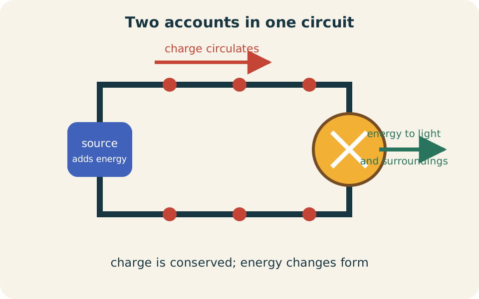
Keep two accounting questions separate throughout the lesson. Ask how much charge crosses a location during an interval, and ask how much energy crosses the boundary of a component. Charge ordinarily circulates through a steady closed circuit and is not consumed by a resistor. Energy is transferred from a source to other stores or surroundings. Confusing those two accounts produces many otherwise avoidable errors.

A circuit requires a closed conducting path

A sustained direct current requires a closed path through which charge can move. A source such as a battery maintains an electric potential difference between its terminals. Conducting connections and components complete the path from one terminal back to the other. Opening a switch interrupts that path and prevents steady current through the break. Voltage may still exist across the open switch even though current is zero there.

Charge is already present throughout a metal conductor before the circuit is connected. Closing the switch establishes an electric field throughout the circuit after electromagnetic changes propagate through the arrangement. Mobile carriers then acquire small net drift velocities superimposed on their rapid microscopic motion. A lamp can respond quickly even though no single electron races from the battery to the lamp at near-light speed. Signal propagation, carrier drift, and energy transport are related but distinct processes.

A circuit diagram suppresses physical shape to emphasize connectivity. Lines represent conducting paths, while symbols represent sources, resistors, switches, and other elements. Points connected by ideal wire are often modeled at the same electric potential. Real wires have some resistance and distributed electromagnetic behavior, but the ideal-wire model is often adequate at introductory scales. Every simplified diagram should be read as a model with stated approximations.

Current measures charge flow rate

Electric current is the rate at which charge crosses an imagined surface. For an instantaneous rate, $I=\frac{dQ}{dt}$. The symbol $I$ denotes current, $Q$ denotes charge in coulombs, and $t$ denotes time in seconds. The derivative describes how rapidly accumulated crossing charge changes at a particular instant. One ampere equals one coulomb per second, so $1\,\mathrm{A}=1\,\frac{\mathrm{C}}{\mathrm{s}}$.

For a constant current over a time interval, the relationship becomes $I=\frac{\Delta Q}{\Delta t}$. Solving gives $\Delta Q=I\Delta t$. The capital Greek delta means final value minus initial value or, in this context, an amount transferred during the interval. Current is not the total charge in the wire. It is a crossing rate measured at a chosen surface.

If current varies with time, transferred charge is $\Delta Q=\int_{t_i}^{t_f}I(t)\,dt$. On a current-versus-time graph, this integral is signed area between the curve and time axis. Positive and negative intervals represent opposite conventional directions. A brief large current and a longer small current can transfer equal charge. The graph therefore contains information that a single peak-current value cannot provide.

Conventional current and electron drift

Conventional current direction is defined as the direction positive charge would move. This convention was established before the electron’s role in metals was known. In a metal, mobile electrons drift opposite conventional current because their charge is negative. Circuit arrows and component sign conventions usually refer to conventional current. The historical convention remains internally consistent when used carefully.

Suppose an electric field points east in a metal wire. A positive carrier would accelerate east, so conventional current points east. An electron experiences force opposite the field and drifts west. Multiplying negative carrier charge by westward drift velocity yields an eastward conventional-current contribution. Thus negative carriers moving west can produce positive current east.

Not all materials use the same mobile carriers. Positive and negative ions can both transport charge in an electrolyte, while holes provide a useful positive-carrier description in semiconductors. Conventional current allows circuit-level reasoning without changing arrow rules for each material. Microscopic interpretation must still identify actual carriers when material behavior matters. The convention is a definition, not a claim that electrons are positive.

Current is not carrier speed

Macroscopic current in a uniform conductor can be modeled as $I=n|q|A v_d$. The symbol $n$ is the number of mobile carriers per cubic meter. The quantity $|q|$ is charge magnitude per carrier in coulombs, $A$ is cross-sectional area in square meters, and $v_d$ is drift-speed magnitude in meters per second. Multiplying these factors yields coulombs per second. This equation connects a circuit measurement with a microscopic model.

A large current does not necessarily require a large drift speed. Metals contain enormous numbers of mobile electrons, so modest drift can transport substantial charge per second. Increasing cross-sectional area also allows more carriers to cross a surface simultaneously. Increasing carrier density or charge magnitude has a similar effect. The equation prevents current from being interpreted as the speed of an individual electron.

The rapid response of a circuit is associated with establishment of an electric field and electromagnetic energy flow, not with one carrier completing the entire loop. A useful analogy is a filled pipe in which pushing at one end produces motion elsewhere before any particular molecule travels the pipe’s length. The analogy is limited because circuit fields and energy reside in three-dimensional space around conductors as well as inside matter. Still, it helps separate collective response from slow net drift. A complete explanation should not imagine empty wires waiting to be filled by a battery.

Voltage measures energy change per charge

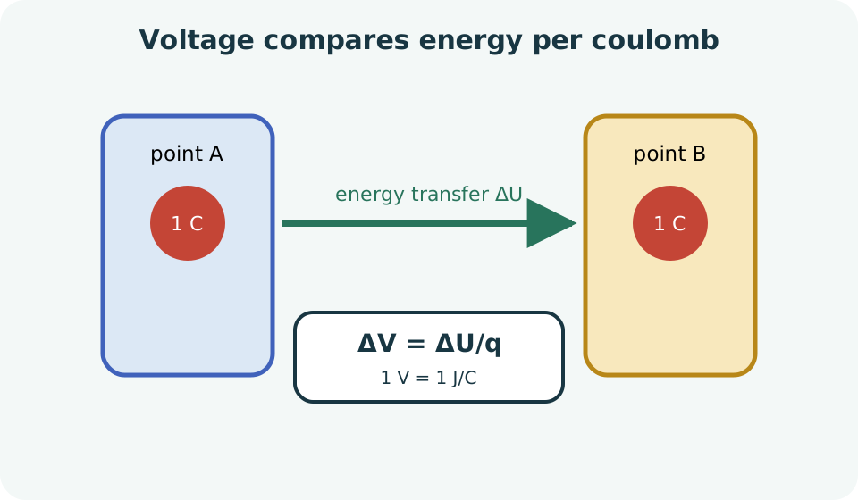
Electric potential difference is defined by $\Delta V=\frac{\Delta U}{q}$. The symbol $\Delta V$ is voltage between two points in volts, and $\Delta U$ is electric potential-energy change in joules for charge $q$ in coulombs. One volt equals one joule per coulomb, so $1\,\mathrm{V}=1\,\frac{\mathrm{J}}{\mathrm{C}}$. Voltage is therefore not energy by itself. It is an energy-per-charge comparison between two locations.

The endpoints and order matter because $\Delta V=V_f-V_i$. Reversing the endpoints reverses the sign of the potential difference. A voltmeter measures potential difference between its two leads rather than voltage “at” one isolated point. Statements such as “this node is at $5\,\mathrm{V}$” implicitly select a reference node assigned zero potential. Potential differences are physically meaningful even though the reference value is chosen.

When charge moves through a source, the source can increase electric potential energy per coulomb. When charge moves through a resistor or lamp, electrical energy is transferred into internal energy, light, or other forms. The same charges continue around a steady circuit. A $12.0\,\mathrm{V}$ source transfers $12.0\,\mathrm{J}$ per coulomb through its internal processes. It does not put twelve coulombs into the circuit.

Resistance compares voltage and current

At a specified operating point, resistance is defined as $R=\frac{\Delta V}{I}$. The symbol $R$ denotes resistance in ohms, written $\Omega$. One ohm equals one volt per ampere, so $1\,\Omega=1\,\frac{\mathrm{V}}{\mathrm{A}}$. Resistance describes how a component relates potential difference and current under stated conditions. It is not a substance that gets used up.

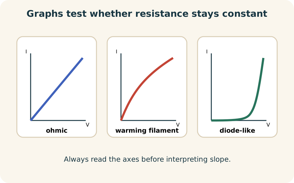
The definition $R=\frac{\Delta V}{I}$ can be applied as a ratio at a measured operating point. Ohm’s law is the stronger claim that $\Delta V=IR$ with constant $R$ across a range of currents under controlled physical conditions. A component with a straight voltage-current graph through the origin is ohmic over that range. A filament lamp, diode, or biological tissue may be nonohmic. Temperature, direction, illumination, and other state variables can affect the relationship.

The language “resistance opposes current” can be useful but incomplete. A resistor does not choose a current independently of the rest of the circuit. The source, network connections, and component characteristics jointly determine the operating point. For a fixed applied voltage in an ohmic component, larger resistance gives smaller current. For a fixed current, larger resistance requires a larger voltage difference.

Voltage-current graphs reveal behavior

A graph can place current $I$ on the vertical axis and voltage $\Delta V$ on the horizontal axis. For an ohmic component obeying $I=\frac{\Delta V}{R}$, the slope is $\frac{1}{R}$. This reciprocal resistance is conductance $G$, measured in siemens. A steeper line therefore represents smaller resistance when current is plotted vertically. Axis order must be checked before interpreting slope.

If voltage is plotted vertically and current horizontally, the slope is instead $R=\frac{\Delta V}{\Delta I}$ for a linear graph. The same physical component now has a steeper line when resistance is larger. Memorizing “slope equals resistance” without checking axes is unreliable. Write the slope as rise over run with units. The units will identify whether it represents ohms or siemens.

A curved graph indicates changing ratio or changing local slope. The ratio $\frac{V}{I}$ is sometimes called static resistance at that point. The local differential resistance is $\frac{dV}{dI}$ when voltage is graphed against current. Those quantities need not be equal for a nonlinear device. Stating which one is used prevents a nonohmic component from being forced into an inappropriate constant-$R$ model.

Resistivity and conductor geometry

For a uniform conductor of length $L$ and cross-sectional area $A$, resistance is modeled by $R=\rho\frac{L}{A}$. The Greek letter $\rho$, pronounced rho, is material resistivity in ohm-meters. Length is measured along the current path in meters. Area is measured perpendicular to current in square meters. This relationship assumes a uniform material and approximately uniform geometry.

Increasing length increases resistance because carriers interact over a longer path. Increasing area decreases resistance because more parallel microscopic pathways are available. Resistivity separates material response from the conductor’s dimensions. Copper has low resistivity and is useful for wiring, while insulating materials have far larger resistivities. Resistivity can vary with temperature and other physical conditions.

Unit analysis confirms the expression. Ohm-meters multiplied by meters and divided by square meters leaves ohms. A common error uses diameter in place of area for a cylindrical wire. The correct area is $A=\pi r^2=\frac{\pi d^2}{4}$, where $r$ is radius and $d$ is diameter. Doubling diameter increases area by a factor of four and therefore reduces resistance by a factor of four when other conditions remain fixed.

Microscopic picture of resistance

An electric field in a conductor exerts forces on mobile carriers. Between interactions with the lattice, defects, or vibrations, carriers acquire a small directed drift. Scattering transfers organized electrical energy into microscopic internal motion of the material. This process contributes to thermal energy and can raise conductor temperature. Resistance summarizes that macroscopic response under specified conditions.

The word collision can be misleading if imagined as classical balls simply bouncing in empty space. Conduction in solids is fundamentally quantum mechanical, and detailed material behavior depends on band structure and scattering processes. The introductory model nevertheless captures a useful causal chain from electric field to drift and energy transfer. It explains why resistance depends on material and temperature. It also clarifies why carriers are not destroyed by a resistor.

For many metals, resistivity increases as temperature rises over ordinary ranges. A hotter lattice has stronger vibrations that enhance scattering. A filament lamp therefore changes resistance substantially as it warms, making its voltage-current graph nonlinear. Some materials behave differently, and superconductors exhibit dramatically different behavior below critical conditions. Constant resistance is a model to test, not an eternal property label.

Electrical power and energy transfer

Power is the rate of energy transfer, so $P=\frac{dE}{dt}$. A component with current $I$ and voltage magnitude $\Delta V$ transfers power at magnitude $P=I\Delta V$. Amperes times volts becomes coulombs per second times joules per coulomb, leaving joules per second. One joule per second is one watt. The equation therefore has both physical and dimensional meaning.

For an ohmic resistor with $\Delta V=IR$, substitution gives $P=I^2R$. Solving Ohm’s law as $I=\frac{\Delta V}{R}$ instead gives $P=\frac{(\Delta V)^2}{R}$. These forms are equivalent only when the same voltage, current, and resistance describe the same ohmic operating point. Choose the form that matches known quantities. Do not infer opposite trends without stating which variable is held fixed.

If current and voltage are constant over time, transferred energy is $E=P\Delta t=I\Delta V\Delta t$. If they vary, energy is the time integral of instantaneous power. A kilowatt-hour is a unit of energy rather than power. One kilowatt-hour equals $(1000\,\mathrm{W})(3600\,\mathrm{s})=3.60\times10^6\,\mathrm{J}$. Energy bills charge for accumulated transfer, not for current alone.

Worked charge and energy account

A device carries $2.00\,\mathrm{A}$ through a potential difference of $12.0\,\mathrm{V}$ for $30.0\,\mathrm{s}$. The transferred charge is $\Delta Q=I\Delta t=(2.00\,\frac{\mathrm{C}}{\mathrm{s}})(30.0\,\mathrm{s})=60.0\,\mathrm{C}$. This calculation answers how much charge crosses a chosen surface. The current is assumed constant over the interval. Significant figures reflect the stated measurements.

Energy transferred is $E=\Delta Q\Delta V=(60.0\,\mathrm{C})(12.0\,\frac{\mathrm{J}}{\mathrm{C}})=720\,\mathrm{J}$. Coulombs cancel, leaving joules. The same result follows from $P=I\Delta V=(2.00\,\mathrm{A})(12.0\,\mathrm{V})=24.0\,\mathrm{W}$. Multiplying by time gives $E=(24.0\,\mathrm{W})(30.0\,\mathrm{s})=720\,\mathrm{J}$. Two calculation paths provide a consistency check.

The $60.0\,\mathrm{C}$ is not consumed by the device. In a steady closed circuit, equal charge per second enters and leaves the device. The $720\,\mathrm{J}$ is energy transferred during the interval, perhaps mainly into internal energy. Distinguishing those statements keeps charge conservation separate from energy transformation. A complete answer names both the calculated quantity and its physical account.

Measuring current and voltage

An ideal ammeter measures current through a branch and is connected in series with that branch. Series placement makes the branch charge flow pass through the meter. An ideal ammeter has zero resistance so it does not alter the current being measured. A real ammeter has small but nonzero resistance. Connecting it directly across a source can create a dangerously large current.

An ideal voltmeter measures potential difference between two points and is connected in parallel across them. It has infinite resistance in the ideal model, so it draws no current. A real voltmeter has large but finite input resistance. Its presence can alter high-resistance circuits through loading. Measurement devices are therefore parts of the circuit rather than invisible observers.

Polarity and direction signs carry information. A negative voltage reading means the meter’s labeled positive lead is at lower potential than its other lead under the selected convention. A negative current reading means actual conventional current is opposite the assumed reference arrow. These signs do not mean the meter has failed. They report how reality compares with the chosen orientation.

Conservation at nodes and around loops

Charge conservation constrains current at a junction. In a steady state, the total conventional current entering a node equals the total leaving it. Otherwise net charge would accumulate continuously at the node. This relationship is Kirchhoff’s junction rule. It follows from charge conservation rather than from Ohm’s law.

Energy conservation constrains potential changes around a closed loop. Returning to the starting point gives zero net potential change after all rises and drops are added with signs. A source can produce a potential rise, while passive elements can produce drops in the chosen traversal direction. This relationship is Kirchhoff’s loop rule. It reflects energy-per-charge accounting around the loop.

The two rules answer different questions. Junction reasoning tracks charge flow, while loop reasoning tracks energy change per charge. Ohm’s law may connect current and voltage for particular elements, but it does not replace either conservation law. More complex circuits require all three kinds of reasoning. Keeping their roles separate makes circuit systems easier to organize.

Common misconceptions and checks

The first misconception says a battery supplies a fixed current. An ideal battery model supplies a specified voltage, while the connected network determines current. Different loads on the same voltage source can draw different currents. Real batteries also have internal resistance and operating limits. Source and load must be analyzed together.

The second misconception says current is used up by each resistor. In steady state, charge cannot disappear inside an ordinary component. A resistor receives electrical energy and transfers it mainly into internal energy. Current can divide among parallel branches, but branch currents recombine consistently with charge conservation. Smaller downstream current in a single unbranched path would imply charge accumulation.

The third misconception treats resistance as always constant. Ohmic behavior is an empirical relationship valid over specified conditions. Temperature changes can alter resistance, and many devices are intentionally nonlinear. Check graph shape, operating range, and material state before using a constant $R$. Units, limiting cases, and conservation laws should then be used to audit the result.

Practice and retrieval

A current of $0.500\,\mathrm{A}$ flows for $8.00\,\mathrm{s}$. Calculate transferred charge with units. Then calculate how many elementary-charge magnitudes this represents using $e=1.602\times10^{-19}\,\mathrm{C}$. Explain why that number does not mean the source permanently loses those electrons in a closed metallic circuit. Identify the assumption made about current during the interval.

A resistor has $9.00\,\mathrm{V}$ across it and carries $3.00\,\mathrm{A}$. Find its operating-point resistance and power. Calculate energy transferred in $2.00\,\mathrm{min}$, first converting time to seconds. State whether constant resistance is needed for the direct calculation $P=I\Delta V$. Explain which additional relationship would require ohmic behavior.

A wire is replaced by one of the same material and length but twice the diameter. Predict the resistance ratio before calculating. Use the area relationship to justify the factor. Then state the current change if the same fixed voltage is applied and both wires remain ohmic at the same temperature. This task links geometry, material behavior, and circuit operation.

Solutions and reasoning

Transferred charge is $\Delta Q=I\Delta t=(0.500\,\frac{\mathrm{C}}{\mathrm{s}})(8.00\,\mathrm{s})=4.00\,\mathrm{C}$. Dividing by elementary-charge magnitude gives $N=\frac{4.00\,\mathrm{C}}{1.602\times10^{-19}\,\mathrm{C}}=2.50\times10^{19}$. This counts charge equivalents crossing the surface. In a closed circuit, carriers circulate and are not permanently consumed by the source. The calculation assumes constant current.

Resistance is $R=\frac{9.00\,\mathrm{V}}{3.00\,\mathrm{A}}=3.00\,\Omega$. Power is $P=I\Delta V=(3.00\,\mathrm{A})(9.00\,\mathrm{V})=27.0\,\mathrm{W}$. Two minutes equals $120\,\mathrm{s}$, so energy is $E=P\Delta t=(27.0\,\mathrm{W})(120\,\mathrm{s})=3.24\times10^3\,\mathrm{J}$. The power relation applies at the operating point without assuming constant resistance. Using $P=I^2R$ or $P=\frac{(\Delta V)^2}{R}$ requires a compatible ohmic relation at that point.

Doubling diameter multiplies cross-sectional area by four because $A\propto d^2$. Since $R=\rho\frac{L}{A}$, the new resistance is one-fourth the original value. Under the same fixed voltage and ohmic conditions, current becomes four times as large. The prediction follows from geometry before numerical substitution. Constant material, length, temperature, and voltage are essential comparison conditions.

Connection forward

Current, voltage, and resistance provide the vocabulary needed for network analysis. Series and parallel circuits show how charge conservation and energy-per-charge conservation constrain multiple components. Equivalent resistance then summarizes a network’s terminal behavior. Those methods become much clearer when voltage is not confused with current. The present lesson therefore supplies concepts that later circuit algorithms depend upon.

The same vocabulary also supports energy analysis in electronics, biological systems, and instrumentation. Real sources possess internal resistance, sensors can be nonlinear, and measuring devices load the systems they observe. These complications do not discard the foundational model. They require its assumptions to be stated and refined. A strong model grows through controlled extensions rather than through unexplained formula replacement.

Carry forward three questions for every circuit element. What current crosses it, what potential difference appears between its terminals, and what energy transfer occurs? Then ask whether its resistance is constant under the operating conditions. Use charge conservation at junctions and energy conservation around loops. With those accounts separated and then connected, circuit reasoning becomes systematic rather than mysterious.