Series and Parallel Circuits

Circuit diagrams encode connections rather than physical drawing scale. Two elements are in series only when the same current must pass through both without branching between them. Two elements are in parallel only when both ends connect to the same pair of nodes. These topological conditions determine current and voltage relationships. Appearance alone can be misleading.

Equivalent resistance replaces a network with one resistor that draws the same terminal current at the same terminal voltage. It does not claim the internal current, voltage, or power distribution disappears. Series resistances add because voltage changes add at common current. Parallel conductances add because branch currents add at common voltage. Conservation supplies both formulas.

This lesson begins with nodes, branches, and loops. It then derives series and parallel equivalents, analyzes power, and reduces mixed networks. Meter placement and real source resistance will expose practical consequences. Worked examples will carry amperes, volts, ohms, and watts explicitly. The goal is to read structure before calculating.

Learning objectives and an opening prediction

After this lesson, you should identify series and parallel connections from nodes. You should derive equivalent resistance formulas from charge and energy conservation. You should calculate branch current, voltage drop, and power. You should reduce mixed series-parallel networks in a justified order. You should also recognize short circuits, source limits, and correct meter placement.

Imagine adding another resistor in series with a battery and existing resistor. Predict the total current under an ideal fixed-voltage source. Equivalent resistance increases, so current decreases. Each series element carries that same reduced current. Source voltage divides across the elements.

Now add the same resistor as a parallel branch instead. Equivalent resistance decreases because another current pathway opens. Total source current increases, while the original branch retains the same voltage under an ideal source. Parallel addition can therefore demand more from the source. The two operations have opposite effects on terminal resistance.

Nodes, branches, and loops define topology

A node is a set of conducting points connected without intervening circuit elements under the ideal-wire model. Every point on one node has the same electric potential. A branch is a path between two nodes containing one or more elements. A loop is a closed route through the network. These definitions make connection claims precise.

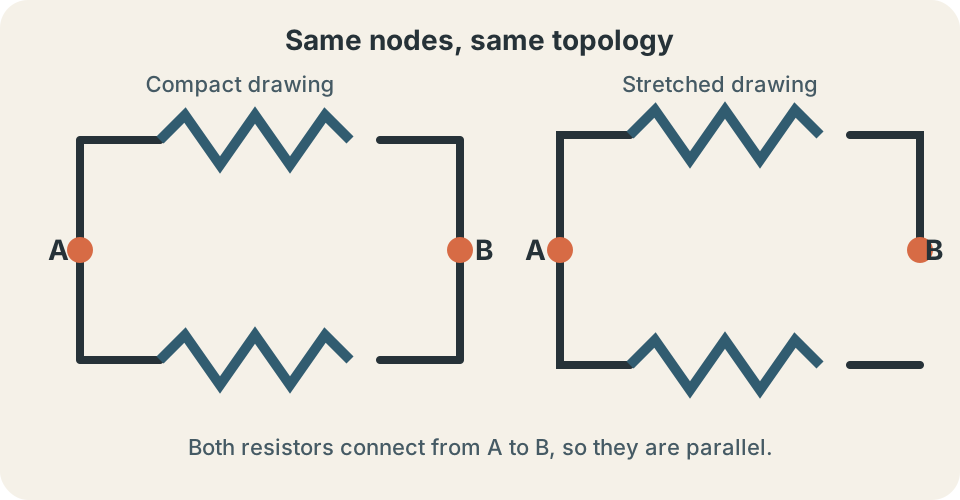
Circuit symbols can be stretched or rearranged without changing topology. A wire drawn with bends remains one node. Crossing lines connect only when the diagram marks a junction according to its notation. Two resistors drawn side by side may not be parallel. Trace their endpoint nodes.

Label major nodes with letters such as A and B. Write each element’s endpoint pair. Elements sharing both endpoint labels are parallel. Elements share guaranteed series current only if their connecting node has no other branch. This node-label method works when visual layouts become complex.

Charge conservation produces the junction rule

In steady operation, charge does not accumulate indefinitely at an ordinary junction. The total current entering equals total current leaving. This is Kirchhoff’s junction rule: $\sum I_{\mathrm{in}}=\sum I_{\mathrm{out}}$. Current is charge flow rate in amperes. The rule expresses charge conservation.

If total current $I$ reaches a node and divides into $I_1$ and $I_2$, then $I=I_1+I_2$. Branch current does not get “used up.” Charge flowing into the junction exits along available paths. Larger branch resistance usually carries smaller current at common voltage. The sum returns when branches rejoin. This equality is the numerical checkpoint at every junction.

Current direction can be assumed. If a solved current is negative, actual direction is opposite the assumed arrow. This is not a failed answer. It is signed accounting. Consistent arrows allow junction equations to reveal direction.

Energy conservation produces the loop rule

As charge moves around a closed loop and returns to its starting point, net electric potential change is zero. Kirchhoff’s loop rule is $\sum\Delta V=0$. Sources raise potential under a chosen traversal, while passive resistors produce drops in the direction of conventional current. Signs depend on traversal and element polarity. A labeled loop prevents guesswork.

For one ideal battery $\mathcal E$ and series resistors, $\mathcal E-IR_1-IR_2-\cdots=0$. Rearranging gives $\mathcal E=I(R_1+R_2+\cdots)$. The source transfers energy per charge, and resistors account for that energy per charge. Voltage is not consumed charge. It is potential-energy change per charge.

The loop and junction rules are more general than series-parallel shortcuts. They can solve bridge networks that cannot be reduced by simple combinations. Equivalent formulas should therefore be understood as consequences of conservation plus element laws. Kirchhoff’s rules provide the foundation. Ohm’s law supplies each resistor’s voltage-current relation.

Series elements share current

Two elements are in series when they lie along one path and their connecting node has no other branch. Charge reaching that internal node has only one way to continue. Steady current through both elements is therefore equal. This common current is a topological consequence. It is not caused by equal resistance.

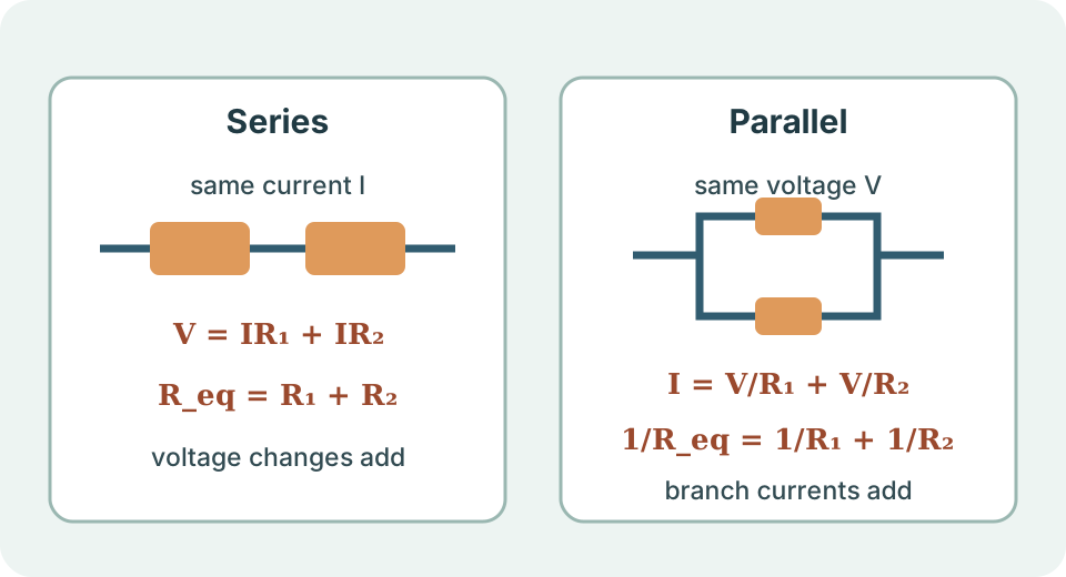
For resistors, write voltage drops $\Delta V_1=IR_1$ and $\Delta V_2=IR_2$. Loop conservation gives terminal voltage $\Delta V=IR_1+IR_2=I(R_1+R_2)$. Define equivalent resistance by $\Delta V=IR_{\mathrm{eq}}$. Thus $R_{\mathrm{eq}}=R_1+R_2$ for two series resistors. The derivation depends on shared current rather than visual alignment.

For many series resistors, $R_{\mathrm{eq}}=\sum_iR_i$. Equivalent resistance exceeds every individual positive resistance. Adding series resistance reduces current for fixed ideal source voltage. Voltage divides in proportion to resistance because $\Delta V_i=IR_i$. The largest resistance has the largest drop at common current.

Worked series example

A $12.0\,\mathrm V$ ideal source connects to $4.00\,\Omega$ and $8.00\,\Omega$ resistors in series. Equivalent resistance is $R_{\mathrm{eq}}=4.00+8.00=12.0\,\Omega$. Source current is $I=\frac{12.0\,\mathrm V}{12.0\,\Omega}=1.00\,\mathrm A$. That same current passes through both resistors. The ohm is volts per ampere.

Voltage drops are $\Delta V_1=(1.00\,\mathrm A)(4.00\,\Omega)=4.00\,\mathrm V$ and $\Delta V_2=(1.00\,\mathrm A)(8.00\,\Omega)=8.00\,\mathrm V$. Their sum is $12.0\,\mathrm V$, matching the source. The larger resistor receives the larger voltage drop. Charge current remains equal. Energy per charge divides.

Power values are $P_1=I^2R_1=4.00\,\mathrm W$ and $P_2=I^2R_2=8.00\,\mathrm W$. Total resistor power is $12.0\,\mathrm W$. Source power is $P_{\mathrm{source}}=I\mathcal E=(1.00)(12.0)=12.0\,\mathrm W$. The power ledger balances. Equal input and output power confirms the ideal energy accounting.

Parallel elements share voltage

Two elements are parallel when their first ends share one node and their second ends share another node. Node potentials fix the same voltage difference across every branch. Their currents need not be equal. Each branch current follows its own element relation. For resistors, $I_i=\frac{\Delta V}{R_i}$.

Junction conservation gives $I=I_1+I_2=\frac{\Delta V}{R_1}+\frac{\Delta V}{R_2}$. Factor voltage: $I=\Delta V\left(\frac{1}{R_1}+\frac{1}{R_2}\right)$. Define $I=\frac{\Delta V}{R_{\mathrm{eq}}}$. Therefore $\frac{1}{R_{\mathrm{eq}}}=\frac{1}{R_1}+\frac{1}{R_2}$. The reciprocal form follows from adding currents at shared voltage.

For two resistors, $R_{\mathrm{eq}}=\frac{R_1R_2}{R_1+R_2}$. Equivalent parallel resistance is smaller than either positive branch resistance. Adding a parallel branch increases total conductance and lowers equivalent resistance. Under fixed voltage, total current increases. This trend checks arithmetic.

Conductance makes parallel addition intuitive

Conductance is $G=\frac{1}{R}$ and is measured in siemens, $\mathrm S=\mathrm{\frac{A}{V}}$. A high-conductance branch carries more current at a given voltage. Parallel conductances add directly: $G_{\mathrm{eq}}=\sum_iG_i$. This mirrors adding available pathways. Equivalent resistance is the reciprocal of total conductance.

If two equal resistors $R$ are in parallel, $G_{\mathrm{eq}}=\frac{1}{R}+\frac{1}{R}=\frac{2}{R}$. Therefore $R_{\mathrm{eq}}=\frac{R}{2}$. Three equal resistors give $\frac{R}{3}$. A result larger than $R$ would contradict the added-pathway interpretation. Equal parallel branches divide current equally.

Conductance is especially useful for many parallel branches. It avoids repeatedly manipulating nested fractions. Electrical power systems and electronic analysis often use related admittance concepts for alternating current. In direct-current resistor networks, reciprocal resistance is enough. Units reveal whether the calculation currently represents resistance or conductance.

Worked parallel example

A $12.0\,\mathrm V$ ideal source connects $6.00\,\Omega$ and $3.00\,\Omega$ resistors in parallel. Reciprocal equivalent is $\frac{1}{R_{\mathrm{eq}}}=\frac{1}{6.00\,\Omega}+\frac{1}{3.00\,\Omega}=\frac{1}{2.00\,\Omega}$. Thus $R_{\mathrm{eq}}=2.00\,\Omega$. It is smaller than $3.00\,\Omega$, as required. Both branches have $12.0\,\mathrm V$ across them.

Branch currents are $I_1=\frac{12.0\,\mathrm V}{6.00\,\Omega}=2.00\,\mathrm A$ and $I_2=\frac{12.0\,\mathrm V}{3.00\,\Omega}=4.00\,\mathrm A$. Total current is $6.00\,\mathrm A$. Equivalent calculation gives $\frac{12.0\,\mathrm V}{2.00\,\Omega}=6.00\,\mathrm A$. Junction current balances. The lower-resistance branch carries twice the current.

Branch powers are $P_1=\frac{(12.0\,\mathrm V)^2}{6.00\,\Omega}=24.0\,\mathrm W$ and $P_2=\frac{(12.0\,\mathrm V)^2}{3.00\,\Omega}=48.0\,\mathrm W$. Total is $72.0\,\mathrm W$. Source power is $(12.0\,\mathrm V)(6.00\,\mathrm A)=72.0\,\mathrm W$. Smaller parallel resistance receives more power at common voltage. The two independent calculations close the power ledger.

Voltage dividers

Two series resistors across an input voltage form a voltage divider. Since current is $I=\frac{V_{\mathrm{in}}}{R_1+R_2}$, output across $R_2$ is $V_{\mathrm{out}}=IR_2=V_{\mathrm{in}}\frac{R_2}{R_1+R_2}$. The horizontal fraction shows the selected resistance over total series resistance. The ratio lies between zero and one for positive resistors. Output is therefore a fraction of input.

If $R_1=2.00\,\mathrm{k\Omega}$ and $R_2=3.00\,\mathrm{k\Omega}$ across $10.0\,\mathrm V$, then $V_{\mathrm{out}}=10.0\frac{3.00}{5.00}=6.00\,\mathrm V$. The kilo-ohm factors cancel in the ratio. Series current is $2.00\,\mathrm{mA}$. The output is measured across the designated resistor. Reversing the resistor positions would change the selected output.

A load connected across $R_2$ changes the circuit because it is parallel with $R_2$. The loaded equivalent becomes $R_2\parallel R_L$, reducing output compared with the unloaded prediction. A real voltmeter also has finite input resistance, though usually high. Voltage-divider formulas require the load assumption. Measurement can alter the system.

Current dividers

Parallel branch current divides according to conductance. For two resistors, total current $I$ splits as $I_1=I\frac{R_2}{R_1+R_2}$ through $R_1$ and $I_2=I\frac{R_1}{R_1+R_2}$ through $R_2$. The opposite resistance appears in each numerator after algebra. Smaller resistance receives larger current. The branch currents sum to $I$.

Derive rather than memorize. Common voltage is $V=IR_{\mathrm{eq}}$. Then $I_1=\frac{V}{R_1}=I\left(\frac{R_{\mathrm{eq}}}{R_1}\right)$. Substituting $R_{\mathrm{eq}}=\frac{R_1R_2}{R_1+R_2}$ yields the divider relation. Conductance fractions provide an even clearer form: $I_1=I\frac{G_1}{G_1+G_2}$.

Current-divider formulas assume only the specified parallel branches share the incoming current. Additional branches alter total conductance. Dependent or nonlinear elements require their own current-voltage laws. Topology alone gives common voltage; element behavior determines division. Verify with the junction sum.

Mixed networks require local reduction

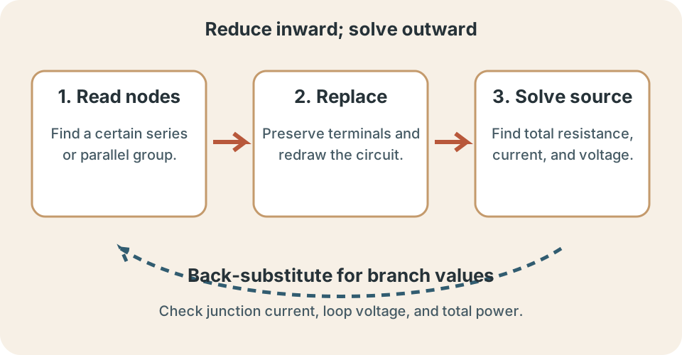
A mixed network contains both series and parallel subgroups. Identify the innermost pair whose relationship is unambiguous. Replace it with an equivalent resistor between the same two nodes. Redraw or relabel the circuit. Continue until one terminal equivalent remains.

Suppose $R_1=4.00\,\Omega$ is in series with a parallel combination of $R_2=6.00\,\Omega$ and $R_3=3.00\,\Omega$. The parallel equivalent is $2.00\,\Omega$. Total equivalent is $4.00+2.00=6.00\,\Omega$. Across $12.0\,\mathrm V$, source current is $2.00\,\mathrm A$. That current passes through $R_1$ before dividing.

Voltage across $R_1$ is $8.00\,\mathrm V$, leaving $4.00\,\mathrm V$ across the parallel group. Branch currents are $\frac{4.00\,\mathrm V}{6.00\,\Omega}=0.667\,\mathrm A$ and $\frac{4.00\,\mathrm V}{3.00\,\Omega}=1.33\,\mathrm A$. Their sum is $2.00\,\mathrm A$ within rounding. Work outward to get the total, then backward to recover internal quantities. The explicit units also confirm that voltage divided by resistance produces current.

Not every circuit is series-parallel reducible

A bridge network can contain resistors that share neither guaranteed current nor both endpoint nodes. No local series or parallel formula applies. Forcing a reduction changes the network. Label nodes before combining. If conditions fail, use Kirchhoff equations or other network methods.

A balanced Wheatstone bridge has a special condition causing zero current through the central branch. Only then can simplification follow from that result. The zero-current claim must be derived from equal node potentials. It is not visually obvious for arbitrary resistance values. Symmetry can help when justified.

Kirchhoff’s rules produce simultaneous linear equations for branch currents or node voltages. Matrix methods solve larger networks. Equivalent resistance can also be found by applying a test voltage and calculating total current. Series-parallel reduction is one tool within a broader framework. Knowing when not to use it is part of mastery.

Short circuits and open circuits

An ideal short circuit has zero resistance between two nodes, making their voltage difference zero. A resistor connected in parallel with an ideal short has zero voltage across it and carries zero current under the ideal resistor model. Current follows the short path, limited only by other circuit resistance. Real wires and sources have nonzero resistance. Short-circuit currents can be dangerous.

An open circuit has no conducting path and effectively infinite resistance in the ideal model. Steady current through that branch is zero. Voltage can still exist across the open terminals. An open switch interrupts current without necessarily removing source voltage. Zero current does not imply zero voltage.

Do not simplify “current takes the path of least resistance” into a claim that no current uses higher-resistance parallel paths. Finite parallel branches all carry current according to common voltage. An ideal zero-resistance branch is a special limiting case. Current divides inversely with resistance, not exclusively in ordinary networks. Quantitative relations replace slogans.

Meters must respect circuit structure

An ammeter measures current through a branch and is placed in series with it. An ideal ammeter has zero resistance. Connecting it directly across a voltage source creates an ideal short and can damage a real meter. Real meters include fuses and small internal resistance. Select a safe current range.

A voltmeter measures potential difference between two nodes and is placed in parallel. An ideal voltmeter has infinite resistance and draws no current. A real voltmeter has high finite resistance. It can load a high-resistance circuit. Measurement diagrams should include the meter as a circuit element when accuracy matters.

An ohmmeter generally applies an internal test signal and must not be connected to an energized circuit unless its instructions permit it. Parallel paths can change the measured equivalent. Components may need isolation from the network. Safe practice follows instrument ratings and circuit de-energization procedures. Classroom idealizations do not override electrical safety.

Real sources have internal resistance

An ideal voltage source maintains fixed terminal voltage for any current, which is physically impossible at unlimited load. Model a real source as emf $\mathcal E$ in series with internal resistance $r$. Terminal voltage while delivering current is $V_{\mathrm{term}}=\mathcal E-Ir$. Greater current produces a larger internal drop. The source also heats internally.

If load resistance is $R_L$, current is $I=\frac{\mathcal E}{r+R_L}$. Load voltage is $IR_L$. As $R_L$ approaches zero, current approaches $\frac{\mathcal E}{r}$ rather than infinity. Internal resistance limits short-circuit current in this simple model. Real protection and electrochemistry add further limits.

Adding parallel loads lowers external equivalent resistance and increases source current. Terminal voltage can then sag. The ideal-source prediction that original branch voltage remains unchanged may fail. Household circuits aim to maintain nearly common voltage while protection limits dangerous total current. Source and wiring constraints matter.

Power depends on the connection constraint

Resistor power can be written $P=IV=I^2R=\frac{V^2}{R}$ for ohmic behavior. In series, current is common, so larger resistance receives larger power $I^2R$. In parallel, voltage is common, so smaller resistance receives larger power $\frac{V^2}{R}$. These conclusions differ because the controlled quantity differs. State topology before comparing.

Equivalent power equals sum of component powers under consistent ideal accounting. For a terminal voltage $V$, total resistor power is $\frac{V^2}{R_{\mathrm{eq}}}$. In parallel, reducing $R_{\mathrm{eq}}$ raises total power demand from an ideal voltage source. In series, increasing $R_{\mathrm{eq}}$ lowers it. Power trends provide a second check on equivalent resistance.

Component power ratings are limits, not predicted operating powers. Calculate actual power and compare with rating using design margin. Resistors can change resistance as they heat. Batteries, wires, and switches also have current and thermal limits. A mathematically valid network can be physically unsafe.

Tolerance and uncertainty

Real resistors have tolerance, such as $\pm1\%$ or $\pm5\%$. Equivalent resistance therefore has a range. In series, worst-case extremes add directly. In parallel, nonlinear reciprocal relationships require recalculation or uncertainty propagation. Measured values may differ from color-code nominal values.

For two independent uncertain series resistors, standard uncertainties can combine in quadrature under an appropriate statistical model. Worst-case engineering bounds instead add absolute extremes. These methods answer different confidence questions. State which is used. Do not report excessive digits from nominal data.

Temperature coefficient changes resistance with operating conditions. Meter uncertainty and lead resistance affect measurement. Contact resistance becomes important for small resistances. Repeat readings and compare with predicted ranges. Disagreement can reveal topology or connection errors.

Common misconceptions and repairs

One misconception says current decreases after each series resistor because the resistor “uses it.” In steady series flow, current is the same everywhere along the unbranched path. Voltage drops account for energy transfer per charge. Charge conservation prevents progressive current loss. A junction is needed for current division. Resistors transform electrical energy without consuming charge.

Another misconception says equal parallel voltage implies equal current. Branch currents depend on resistance. Equal resistances share equally; unequal resistances do not. Apply $I=\frac{V}{R}$ to each branch. Then verify the sum.

A third misconception combines resistors based on visual proximity. Series requires a branch-free shared node, and parallel requires the same two endpoint nodes. Label nodes. Redraw without changing connections. Topology, not page layout, decides the formula.

Practice with guided feedback

First, find equivalent resistance of $10.0\,\Omega$ and $15.0\,\Omega$ in series. Second, find their parallel equivalent. Third, place each combination across $12.0\,\mathrm V$ and find total current. Fourth, explain why the parallel current is larger. Include units and trend checks.

Series equivalent is $25.0\,\Omega$, giving $I=\frac{12.0}{25.0}=0.480\,\mathrm A$. Parallel equivalent is $\frac{(10.0)(15.0)}{10.0+15.0}=6.00\,\Omega$, giving $I=2.00\,\mathrm A$. Parallel current is larger because equivalent resistance is lower at the same voltage. Added conductance supplies an additional branch. Both results fit their inequalities.

For a topology check, mark all nodes. For a conservation check, sum branch currents and loop voltage changes. For a power check, compare source power with resistor totals. For a meter check, place ammeters in series and voltmeters across nodes. These four checks expose most circuit errors.

Retrieval and connection forward

Without looking back, define node, branch, loop, series, and parallel. Derive both equivalent-resistance formulas from conservation and Ohm’s law. Solve a mixed network outward and then recover internal values backward. Explain open and short circuits. Finish by balancing charge, voltage, and power.

Kirchhoff’s rules will solve networks beyond simple reduction. Capacitors will show different series and parallel relationships because stored charge and voltage constraints differ. Alternating-current circuits replace resistance with impedance. Electronics introduces nonlinear devices and operating points. Topology and conservation remain foundational.

Keep one organizing statement: series elements share current because there is no branch, while parallel elements share voltage because they connect to the same nodes. Voltage changes add in loops and currents add at junctions. Equivalent resistance preserves terminal behavior, not internal details. Power, meter loading, source resistance, and component limits complete the physical circuit story. Every reliable solution returns to topology and conservation.