Ohm’s Law

Ohm’s law describes a remarkably useful pattern: for some circuit elements under stable physical conditions, voltage difference is proportional to current. Doubling the voltage across such an element doubles its current. The proportionality constant is resistance. This statement is an empirical material model rather than a universal command that every device must obey. Lamps, diodes, thermistors, and biological tissue can behave differently.

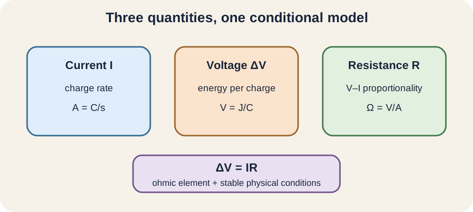
Three electrical quantities must remain conceptually separate. Current describes the rate of charge flow, voltage difference describes energy transferred per unit charge, and resistance describes opposition encoded by an element’s voltage–current relationship. The equation connects them but does not make them interchangeable. Units provide their operational meanings. Amperes, volts, and ohms must accompany every numerical result.

This lesson begins with measurement and graphs before manipulating formulas. It then connects resistance to material and geometry, derives power relationships, and examines temperature effects. Non-ohmic curves will reveal the limits of the linear model. Worked examples will use explicit polarity and current direction. The goal is to read a circuit as a physical system, not merely cover two letters in a formula triangle.

Learning objectives and an opening prediction

After this lesson, you should state the conditions under which Ohm’s law applies. You should distinguish the definition of instantaneous or static resistance from the claim that resistance is constant. You should obtain resistance or conductance from correctly oriented graphs. You should calculate current, voltage, resistance, and power with appropriate units. You should also design a basic measurement and recognize non-ohmic behavior.

Imagine measuring an unknown device at several applied voltages. The points on a voltage-versus-current graph fall on a straight line through the origin. Predict what happens when current doubles. The voltage difference doubles, while the ratio of voltage to current remains fixed. The slope of that graph is the device’s resistance under the tested conditions.

Now imagine the graph bends upward as current increases. The ratio $\frac{V}{I}$ is no longer constant across operating points. Ohm’s law with one constant resistance does not describe the full curve. One may still calculate a ratio at a chosen point, but that number does not predict every other point. The distinction between a local description and a global linear model is essential.

Current and voltage are different physical quantities

Electric current is $I=\frac{\Delta q}{\Delta t}$ for an average interval or $I=\frac{dq}{dt}$ instantaneously. The symbol $I$ denotes current, $q$ is charge in coulombs, and $t$ is time in seconds. One ampere is one coulomb per second, $1\,\mathrm A=1\,\mathrm{\frac{C}{s}}$. Conventional current points in the direction positive charge would move. Electron drift in a metal points oppositely.

Voltage difference is $\Delta V=\frac{\Delta U}{q}$ in an energy-per-charge sense. The symbol $U$ denotes electric potential energy in joules. One volt is one joule per coulomb, $1\,\mathrm V=1\,\mathrm{\frac{J}{C}}$. Voltage is measured between two points and therefore needs a polarity or ordered pair. Saying a point “has voltage” is shorthand relative to a chosen reference.

A battery can maintain a voltage difference even when an open circuit carries no steady current. Closing a conducting path allows current according to the full circuit’s resistance and source behavior. Thus voltage is not “used-up current,” and current is not stored inside a resistor. Energy is transferred from source to circuit elements while charge circulates. A correct model tracks charge conservation and energy transfer separately.

Ohm’s law is a constitutive model

For an ohmic element, $\Delta V=IR$. Here $\Delta V$ is the voltage difference across the element in volts, $I$ is current through it in amperes, and $R$ is resistance in ohms. One ohm is one volt per ampere, $1\,\Omega=1\,\mathrm{\frac{V}{A}}$. The equation says voltage and current are proportional when $R$ remains constant. Physical conditions such as temperature must be sufficiently stable.

Solving algebraically gives $I=\frac{\Delta V}{R}$ and $R=\frac{\Delta V}{I}$. These forms contain the same relationship. The horizontal fraction bar groups the entire voltage difference over resistance or current. Choosing a form should follow the unknown quantity, not a memorized visual trick. Units should be substituted before arithmetic.

Resistance can be defined as the ratio $\frac{\Delta V}{I}$ at a nonzero operating point, but Ohmic behavior makes the stronger claim that this ratio is constant across a range. A diode can have a voltage-to-current ratio at one point without having a single constant $R$. Differential resistance, $r=\frac{dV}{dI}$, describes the local slope of a nonlinear curve. The derivative uses an infinitesimal voltage change over an infinitesimal current change near one operating point. Static and differential resistance answer different questions.

Graphs reveal the model directly

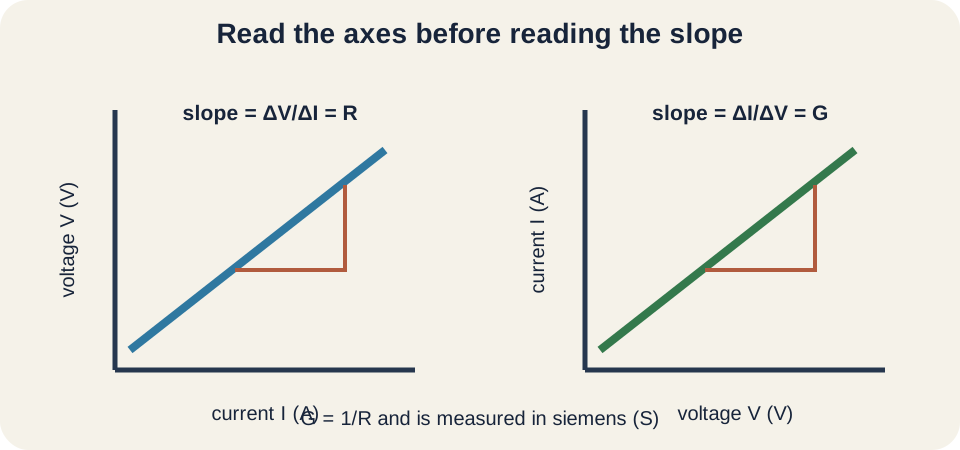
On a graph with voltage $V$ on the vertical axis and current $I$ on the horizontal axis, slope is $\frac{\Delta V}{\Delta I}$. For an ohmic element, that slope equals resistance $R$. A steeper line therefore represents greater resistance. The intercept should be near zero for a passive ideal resistor. A significant intercept or curvature signals another behavior or a measurement issue.

If axes are reversed, current is vertical and voltage is horizontal. The slope is then $\frac{\Delta I}{\Delta V}=\frac{1}{R}$. This reciprocal is conductance, conventionally $G$, measured in siemens. One siemens is one ampere per volt. Axis labels, not graph appearance alone, determine the physical slope.

Use widely separated points on a best-fit line rather than two adjacent noisy measurements. Subtract coordinates to obtain changes, not raw coordinate ratios unless the fit is constrained through the origin. Include slope units, such as $\mathrm{\frac{V}{A}}=\Omega$. Residuals can reveal systematic curvature that a high correlation coefficient hides. Graphical analysis tests the model rather than merely decorating the data.

Measuring an element safely

An ammeter measures current and is placed in series so the same branch current passes through it. An ideal ammeter has negligible resistance to avoid changing the current. A voltmeter measures potential difference and is connected in parallel across the element. An ideal voltmeter has extremely large resistance to draw negligible current. Reversing these placements can strongly disturb or damage a circuit.

A practical measurement uses a variable source or series limiting resistor. Increase the applied voltage in controlled steps and record current only within component and meter ratings. Allow temperature to stabilize if the goal is constant-temperature resistance. Reverse polarity when appropriate to test symmetry. Repeat measurements to estimate variability.

Meter specifications matter. Real ammeters have burden voltage, real voltmeters have finite input resistance, and leads have resistance. Resolution limits how finely values can be read, while calibration affects accuracy. Uncertainty should be represented in data and, when useful, error bars. A straight line within uncertainty is stronger evidence than visually aligned rounded values.

Worked example: an operating resistor

A $24.0\,\Omega$ resistor is connected across an ideal $12.0\,\mathrm V$ source. Current is $I=\frac{12.0\,\mathrm V}{24.0\,\Omega}=0.500\,\mathrm A$. The ohm unit is $\mathrm{\frac{V}{A}}$, so volts divided by ohms reduce to amperes. Three significant figures follow the stated values. This calculation assumes resistance remains $24.0\,\Omega$ at the resulting temperature.

During $30.0\,\mathrm s$, charge passing a cross-section is $\Delta q=I\Delta t=(0.500\,\mathrm A)(30.0\,\mathrm s)=15.0\,\mathrm C$. The ampere-second reduces to coulombs. This does not mean the resistor contains or consumes $15.0\,\mathrm C$. It means that amount of charge crosses the chosen section during the interval. In a steady circuit, equal charge rates enter and leave.

If voltage doubles to $24.0\,\mathrm V$ while resistance stays constant, current doubles to $1.00\,\mathrm A$. This proportional response is the defining prediction of the ohmic model. In a real resistor, greater current can heat the material and change $R$. The resulting deviation belongs to changing conditions rather than an algebra failure. A short measurement or temperature-controlled bath may be needed to test proportionality independently of self-heating.

Resistance depends on geometry and material

For a uniform conductor, $R=\rho\frac{L}{A}$. The Greek lowercase rho, $\rho$, denotes resistivity in ohm-meters, $L$ is conductor length in meters, and $A$ is cross-sectional area in square meters. Longer conductors have greater resistance because charge carriers encounter a longer path. Larger cross-sectional area provides more parallel microscopic pathways. Resistivity describes material response under specified conditions.

Check the units: $\left(\Omega\,\mathrm m\right)\frac{\mathrm m}{\mathrm{m^2}}=\Omega$. Doubling length doubles resistance when $\rho$ and $A$ remain fixed. Doubling wire diameter multiplies area by four because $A=\pi\frac{d^2}{4}$. Resistance therefore falls by a factor of four. Confusing diameter with area gives an incorrect factor of two.

Resistivity is not resistance. Two copper wires can have different resistances because their lengths or areas differ while their resistivities are nearly the same at equal temperature. Conversely, identical geometry made from different materials can yield different resistance. Contact resistance and nonuniform shape can make the simple formula incomplete. Geometry, material, and interfaces must be specified.

Temperature can change resistance

For many metals over a moderate temperature range, resistance is approximated by $R=R_0[1+\alpha(T-T_0)]$. Here $R_0$ is resistance at reference temperature $T_0$, $T$ is the new temperature, and $\alpha$ is the temperature coefficient in inverse kelvins. The bracketed factor is dimensionless. A positive $\alpha$ means resistance increases with temperature. The linear equation is a local approximation.

Heating a metal increases lattice vibration and typically increases carrier scattering. As current heats a filament, its resistance rises. A tungsten lamp therefore has much lower cold resistance than its steady glowing resistance. Its voltage–current curve bends because physical conditions change with operating point. Treating it as one fixed resistor can seriously underestimate startup current.

Semiconductors and thermistors can have negative temperature coefficients over useful ranges. Their carrier populations and transport mechanisms differ from simple metals. Temperature sensors deliberately exploit predictable resistance changes. Superconductors exhibit a transition to extremely small resistance below a critical temperature under appropriate conditions. No universal sign rule replaces material data.

Electrical power follows energy transfer

Electrical power is $P=I\Delta V$. The symbol $P$ denotes energy-transfer rate in watts, and $1\,\mathrm W=1\,\mathrm{\frac{J}{s}}$. Current gives coulombs per second and voltage gives joules per coulomb, so their product gives joules per second. Under the passive sign convention, positive $P$ means the element receives electrical energy. A source delivering energy may have negative absorbed power under the same convention.

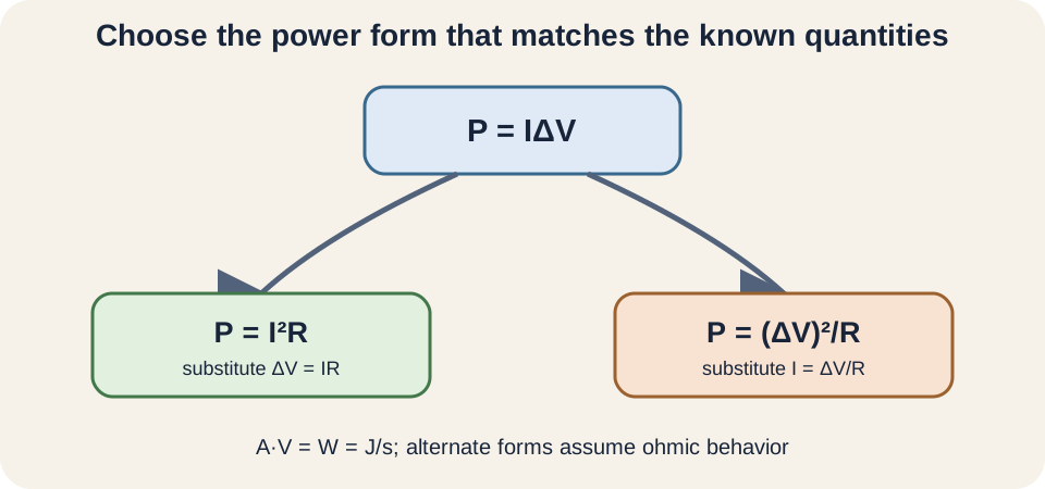
For an ohmic resistor, substitute $\Delta V=IR$ to obtain $P=I^2R$. Alternatively substitute $I=\frac{\Delta V}{R}$ to obtain $P=\frac{(\Delta V)^2}{R}$. These are not three independent laws. They are algebraically equivalent only when the element obeys the relevant Ohm’s-law model. Choose the form that matches known quantities and circuit constraints.

For the $24.0\,\Omega$ resistor at $12.0\,\mathrm V$, $P=(0.500\,\mathrm A)(12.0\,\mathrm V)=6.00\,\mathrm W$. Over $30.0\,\mathrm s$, transferred energy is $E=P\Delta t=(6.00\,\mathrm W)(30.0\,\mathrm s)=180\,\mathrm J$. A resistor rated below $6.00\,\mathrm W$ may overheat. Thermal surroundings determine how hot it ultimately becomes. Power rating is a safety limit, not the resistance value.

Circuit constraints change how power scales

The statement “larger resistance means larger power” is incomplete. If current is held fixed, $P=I^2R$ shows that greater resistance produces greater power. If voltage is held fixed, $P=\frac{V^2}{R}$ shows that greater resistance produces less power. The apparent contradiction disappears when the controlled variable is named. Circuit context determines which comparison applies.

In series, elements carry the same current. Under that constraint, the larger resistance dissipates more power. In parallel across an ideal source, elements share the same voltage. Under that constraint, the smaller resistance dissipates more power. These results follow from the same power equations. Never compare resistance alone without specifying connection and source behavior.

Real sources have internal resistance and limited power. Adding a load can reduce terminal voltage rather than holding it fixed. Maximum power transfer and efficiency then require a source model. Batteries also change voltage with charge state, temperature, and current. The ideal-source examples are useful baselines whose assumptions must remain visible.

Non-ohmic devices carry information

A diode passes substantial current more readily in one direction than the other. Its current–voltage curve is asymmetric and nonlinear. A filament lamp bends because temperature rises with current. A thermistor intentionally changes resistance with temperature. Non-ohmic behavior is not defective behavior; it is often the function of the device.

For a nonlinear device, the operating point is one pair $(V,I)$ determined by both the device curve and external circuit. Static resistance at that point is $R_{\mathrm{static}}=\frac{V}{I}$. Differential resistance is $r=\frac{dV}{dI}$, the tangent slope on a $V$-versus-$I$ graph. Those values may differ greatly. Small-signal circuit response uses the local differential value.

Graph scale can conceal curvature. A broad axis range may make a mildly nonlinear curve appear straight. Residual plots and repeated measurements across the intended operating range provide stronger evidence. Hysteresis, in which the path depends on history, requires measurements while increasing and decreasing drive. Model validation includes range, direction, temperature, and timescale.

Common misconceptions and repairs

One misconception says resistance consumes current. In a steady series circuit, the same current passes through each element. A resistor transfers electrical energy to thermal energy and establishes a voltage drop under the chosen sign convention. Charge does not steadily accumulate inside it. Kirchhoff’s current rule will formalize this conservation.

Another misconception says a battery supplies constant current. An ideal voltage source sets voltage, while current depends on the connected circuit. A short circuit can demand dangerously large current limited by internal and wire resistance. A current-regulated source is a different device model. Always identify what the source holds approximately constant.

A third misconception assumes every ratio $V/I$ proves Ohm’s law. One operating point always supplies a ratio when current is nonzero. Ohmic behavior requires proportionality across a range under controlled conditions. A straight line through the origin is the graphical signature. Multiple measurements, not a single division, test the claim.

Practice with guided feedback

First, find current through $10.0\,\Omega$ at $5.00\,\mathrm V$. Second, find the power received by that resistor. Third, determine the resistance represented by a $V$-versus-$I$ line rising from $(0,0)$ to $(0.400\,\mathrm A,8.00\,\mathrm V)$. Fourth, explain how the answer changes if the graph axes are reversed. Include units at every step.

Current is $I=\frac{5.00\,\mathrm V}{10.0\,\Omega}=0.500\,\mathrm A$. Power is $P=I\Delta V=(0.500\,\mathrm A)(5.00\,\mathrm V)=2.50\,\mathrm W$. The graph slope is $R=\frac{8.00\,\mathrm V}{0.400\,\mathrm A}=20.0\,\Omega$. With current vertical, slope would be conductance $G=\frac{1}{20.0\,\Omega}=0.0500\,\mathrm S$. Axis order determines whether slope is resistance or its reciprocal.

For an experiment-design check, place the ammeter in series and voltmeter in parallel. Limit current so the component remains within its rating. Record multiple operating points and include uncertainty. Plot both a fitted line and residuals. Conclude Ohmic behavior only over the range supported by evidence.

Retrieval and connection forward

Without looking back, define current, voltage difference, resistance, and power in words and units. State Ohm’s law with its physical conditions. Explain what slopes mean on both possible graph orientations. Derive the two alternate resistor-power expressions. Finish by explaining why a lamp’s rising temperature can curve its graph.

Series and parallel lessons will apply charge and energy conservation to networks. Kirchhoff’s rules will formalize junction currents and loop voltage changes. Capacitors will introduce time-dependent current even with constant source voltage. Semiconductor lessons will make nonlinear device curves central. The habits developed here—identify the model, constraint, operating range, and units—transfer to each topic.

Keep one final statement: Ohm’s law is the claim that voltage and current are proportional for an element under stable conditions. Resistance is the proportionality constant and graph slope when voltage is vertical. Power describes energy transfer per time, not charge loss. Geometry, material, and temperature determine resistance. Measurements across a range decide whether the constant-resistance model is justified.