Kirchhoff’s Rules

Simple series and parallel reductions are valuable, but many useful circuits cannot be reduced by inspection. Kirchhoff’s rules provide a systematic language for such networks by applying charge conservation at junctions and energy-per-charge accounting around closed paths. The rules do not replace Ohm’s law; they coordinate component relations such as $\Delta V=IR$ across an entire network. Their power comes from careful definitions, consistent signs, and an explicit circuit model. This lesson develops those habits so that simultaneous equations represent physical reasoning rather than a collection of memorized sign tricks.

Read a circuit as a network

A circuit diagram represents components connected by conducting nodes and branches. A node is a set of points joined by ideal wire and therefore treated as having one electric potential. A branch is a path between nodes that carries one branch current through its series elements. A junction is a node where three or more branch paths meet. Recognizing this topology is the first step because Kirchhoff equations are written from connections, not from the visual shape of the drawing.

Current $I$ is the rate at which charge crosses a chosen surface, $I=\dfrac{\Delta Q}{\Delta t}$. The symbol $Q$ denotes electric charge in coulombs, $t$ denotes time in seconds, and current is measured in amperes. One ampere equals one coulomb per second, written $1\,\mathrm{A}=1\,\mathrm{\dfrac{C}{s}}$. Conventional current direction is defined as the direction positive charge would move. Electron drift in a metal is ordinarily opposite conventional current, but circuit equations use the conventional definition consistently.

Electric potential difference $\Delta V$ is energy change per unit charge. One volt equals one joule per coulomb, $1\,\mathrm{V}=1\,\mathrm{\dfrac{J}{C}}$. A source can raise electric potential, while a resistor traversed in the current direction lowers it. The actual change depends on which way a path crosses the component. Kirchhoff’s loop rule tracks these signed changes around a closed traversal.

Derive the junction rule from charge conservation

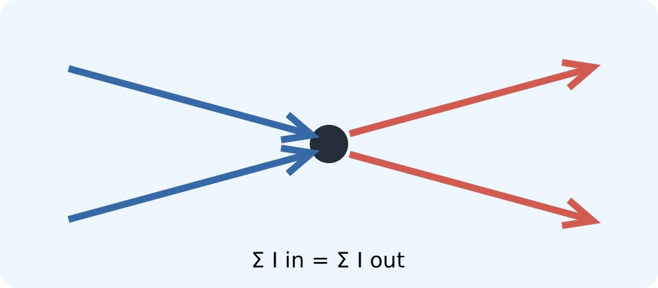
Choose a small boundary enclosing one junction. Charge conservation says that the change in charge stored inside equals charge entering per time minus charge leaving per time. In steady direct-current operation, the junction does not accumulate macroscopic charge, so its stored charge remains constant. The current balance is therefore $\sum I_{\mathrm{in}}=\sum I_{\mathrm{out}}$. Each sigma means to add all branch currents in the indicated category.

An equivalent signed form is $\sum_k s_kI_k=0$, where $s_k=+1$ may be assigned to incoming currents and $s_k=-1$ to outgoing currents. The index $k$ labels the branches connected to the junction. A different sign convention works equally well if used consistently. The equation concerns algebraic current, not the number of wire segments shown. At any node, all inflow must be matched by outflow when the steady-state assumption holds.

Suppose $3.00\,\mathrm{A}$ and $2.00\,\mathrm{A}$ enter a junction, while $1.00\,\mathrm{A}$ and an unknown $I$ leave. The junction equation is $3.00\,\mathrm{A}+2.00\,\mathrm{A}=1.00\,\mathrm{A}+I$. Solving gives $I=4.00\,\mathrm{A}$ outward. Ampere units appear on every term because only quantities with the same dimensions can be added. A quick check confirms $5.00\,\mathrm{A}$ enters and $5.00\,\mathrm{A}$ leaves.

Assign current directions without guessing the answer

Before solving, draw one arrow for each unknown branch current. These arrows are reference directions, not claims about the physical answer. Assigning them arbitrarily is legitimate because the algebra can return a negative value. If $I=-0.500\,\mathrm{A}$ relative to an arrow drawn rightward, the actual conventional current is $0.500\,\mathrm{A}$ leftward. The negative sign corrects the assumption rather than indicating an impossible current.

Do not reverse an arrow midway through the algebra merely because an intermediate expression looks negative. Every resistor sign and junction term was written relative to the original arrow. Changing it silently alters the meanings of earlier equations. Finish the linear system first, then translate negative solutions into actual directions in the final interpretation. Consistent references are more important than initially choosing the “right” direction.

Current is the same through components in one uninterrupted series branch because no intermediate junction permits sustained accumulation. Different branches between the same pair of nodes can carry different currents. Labeling every resistor with a separate unknown when several lie in one series branch creates unnecessary variables. Conversely, assigning one current to components separated by a junction incorrectly suppresses real branch freedom. Topology determines how many independent branch currents the model needs.

Derive the loop rule from energy accounting

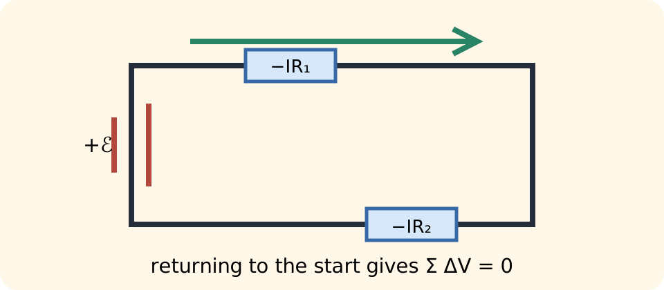
Electric potential is a property assigned to circuit nodes under the lumped, quasistatic model. After traversing any closed loop and returning to the starting node, the net potential change must be zero. Kirchhoff’s loop rule is therefore $\sum\Delta V=0$. The sum includes every signed rise and drop encountered along the chosen traversal. Multiplying the equation by a charge would express the corresponding energy changes for that charge.

The starting point and traversal direction are arbitrary. Going clockwise instead of counterclockwise multiplies every term by $-1$, producing an equivalent equation. Begin at a marked point, move around the loop once, and record each component crossing in sequence. Do not assign signs from a vague rule that sources are positive and resistors are negative. Signs depend on the relationship between traversal direction, terminal labels, and assumed current.

The rule is an energy-per-charge statement within its model assumptions. It does not say that potential is consumed or that current loses energy. Charges transfer energy to components while the steady current continues through them. A resistor converts electrical energy into thermal energy at rate $P=I^2R$, while a source can supply electrical energy. Language should preserve the distinction among charge flow, potential difference, and energy transfer.

Apply component sign conventions

An ideal source is labeled with positive and negative terminals and emf $\mathcal{E}$. The script symbol $\mathcal{E}$ denotes energy supplied per unit charge and is measured in volts. Crossing from the negative terminal to the positive terminal is a rise $+\mathcal{E}$. Crossing from positive to negative is a drop $-\mathcal{E}$. The sign depends only on traversal across the labeled terminals.

For a resistor carrying assumed current $I$, Ohm’s law gives a potential drop of magnitude $IR$ in the current direction. Traversing the resistor with the current contributes $-IR$, while traversing against the current contributes $+IR$. The resistance $R$ is measured in ohms, with $1\,\Omega=1\,\mathrm{\dfrac{V}{A}}$. Thus amperes times ohms reduce to volts, as every term in a loop equation must. If the solved current is negative, the algebra automatically reverses the physical drop relative to the assumed arrow.

A real battery may be modeled as an ideal emf in series with internal resistance $r$. When it delivers current through its positive terminal, its terminal voltage is $V_{\mathrm{term}}=\mathcal{E}-Ir$. When an external source drives charging current into the positive terminal, the relevant sign changes and terminal voltage can exceed emf. The same traversal rules handle both cases without a separate memorized slogan. Draw the internal resistor and apply the ordinary component rules.

Solve a single loop carefully

Consider a loop containing $R_1=4.00\,\Omega$, $R_2=6.00\,\Omega$, a $12.0\,\mathrm{V}$ source aiding clockwise current, and a $2.00\,\mathrm{V}$ source opposing it. Assume current $I$ clockwise and traverse clockwise. The loop equation is $12.0\,\mathrm{V}-2.00\,\mathrm{V}-I(4.00\,\Omega)-I(6.00\,\Omega)=0$. Combining terms gives $10.0\,\mathrm{V}-I(10.00\,\Omega)=0$. Solving yields $I=1.00\,\mathrm{A}$ clockwise.

The result can be checked with units and energy rate. The sources provide a net rise of $10.0\,\mathrm{V}$. The resistor drops are $(1.00\,\mathrm{A})(4.00\,\Omega)=4.00\,\mathrm{V}$ and $(1.00\,\mathrm{A})(6.00\,\Omega)=6.00\,\mathrm{V}$. Their sum is $10.00\,\mathrm{V}$ within the reported precision. Traversing in the opposite direction would produce the negative of the entire original equation and the same current.

Power offers another check. The aiding source supplies $P=(12.0\,\mathrm{V})(1.00\,\mathrm{A})=12.0\,\mathrm{W}$, while the opposing source absorbs $2.00\,\mathrm{W}$. The resistors absorb $I^2(R_1+R_2)=(1.00\,\mathrm{A})^2(10.00\,\Omega)=10.0\,\mathrm{W}$. Total supplied power equals total absorbed power. This check can reveal a sign error that a plausible current magnitude might hide.

Construct a two-loop system

In a multi-loop circuit, choose a current for each independent branch rather than automatically assigning one current per drawn loop. Suppose left and right branches share a central resistor. Label the left branch current $I_1$, the right branch current $I_2$, and determine the central current from a junction equation. Depending on arrow choices, the central current may be $I_1-I_2$, $I_1+I_2$, or another signed relation. A labeled diagram must precede the equations.

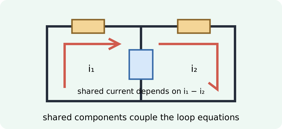
As a concrete system, let a $12.0\,\mathrm{V}$ source and $2.00\,\Omega$ resistor occupy the left branch, a $6.00\,\mathrm{V}$ source and $4.00\,\Omega$ resistor occupy the right branch, and a $3.00\,\Omega$ resistor be shared. Choose clockwise mesh currents $i_1$ in the left loop and $i_2$ in the right loop. In the shared resistor they oppose, so its downward reference current can be $i_1-i_2$. Traversing each mesh in its assigned clockwise direction keeps the sign logic visible. The loop equations become $12.0\,\mathrm{V}-(2.00\,\Omega)i_1-(3.00\,\Omega)(i_1-i_2)=0$ and $6.00\,\mathrm{V}-(4.00\,\Omega)i_2-(3.00\,\Omega)(i_2-i_1)=0$ for compatible source orientations.

Simplification gives $(5.00\,\Omega)i_1-(3.00\,\Omega)i_2=12.0\,\mathrm{V}$ and $-(3.00\,\Omega)i_1+(7.00\,\Omega)i_2=6.00\,\mathrm{V}$. Solving the simultaneous equations gives $i_1=4.25\,\mathrm{A}$ and $i_2=2.68\,\mathrm{A}$ to three significant figures. The shared-branch current is $i_1-i_2=1.57\,\mathrm{A}$ in the $i_1$ reference direction. Substitute both values into both original loop equations and the junction relationship. A solution is not complete until it satisfies every defining equation within rounding.

Choose independent equations

One can trace many closed paths through a network, but not every loop equation adds new information. If one loop equation can be formed by adding or subtracting others, it is dependent. Solving with redundant equations wastes work and may obscure which constraints determine the unknowns. Choose enough independent junction and loop equations to match the number of independent branch-current unknowns. Linear algebra describes this requirement as matching the system’s rank.

For a connected network with $B$ branches and $N$ nodes, there are $N-1$ independent node equations. One node equation is redundant because summing all node balances produces zero automatically. The number of independent loops is $B-N+1$. Together these counts provide $B$ independent equations for $B$ branch currents under typical conditions. This graph-theoretic result explains rather than merely prescribes the usual equation count.

Mesh-current analysis and node-voltage analysis are alternative systematic methods built from the same conservation principles. Mesh analysis assigns currents to independent planar loops and can reduce unknowns when relatively few loops exist. Node-voltage analysis assigns potentials relative to a reference node and can be more efficient for many branches. Kirchhoff’s laws support both methods. The best representation is the one that makes the network constraints easiest to express and verify.

Solve the linear algebra transparently

After equations are written, collect coefficients in a consistent variable order. A system can be represented as $A\mathbf{x}=\mathbf{b}$, where $A$ is the coefficient matrix, $\mathbf{x}$ is the vector of unknown currents, and $\mathbf{b}$ contains source-voltage terms. Matrix form separates circuit modeling from equation solving. Row reduction, substitution, elimination, or software can then solve the same system. The physical challenge is constructing $A$ and $\mathbf{b}$ correctly.

Keep units visible during hand calculations even when the coefficient matrix is written numerically. A resistance coefficient multiplying current produces voltage. Adding a current term directly to a voltage term would be dimensionally invalid. If using software, document the units assigned to every input and output because a numerical solver cannot detect a consistent unit mistake. Dimensional reasoning remains a human responsibility.

Negative solutions should be interpreted, not “fixed” by absolute values. A negative current says that the physical direction is opposite the reference arrow. Reversing the final arrow and reporting the positive magnitude is acceptable if the reinterpretation is explicit. Component power signs should then be recalculated with the actual direction and terminal convention. The algebraic sign contains information that should not be discarded prematurely.

Verify voltage, current, and power

A junction check substitutes solved currents into every relevant node balance. The total incoming current should equal the total outgoing current within rounding. A loop check walks through each independent loop and confirms that signed voltage changes sum to zero. These checks test different conservation relationships. Passing one does not guarantee that the other was modeled correctly.

For a resistor, absorbed power is $P_R=I^2R=VI=\dfrac{V^2}{R}$ when $V$ is the magnitude of its drop. Each form has units of watts, where $1\,\mathrm{W}=1\,\mathrm{\dfrac{J}{s}}=1\,\mathrm{V\,A}$. The squared-current form is nonnegative because an ideal resistor converts electrical energy to thermal energy. For a source, the sign of $P=VI$ depends on whether conventional current enters its positive or negative terminal. The passive sign convention treats current entering a positive-labeled terminal as positive absorbed power.

Summing signed power over all components should give zero in a steady ideal network. Equivalently, total supplied power equals total absorbed power. A mismatch often reveals a reversed source contribution, an incorrect shared-branch current, or a copied arithmetic value. Small discrepancies can arise from rounding, so retain extra digits during intermediate steps. Power balance is an independent physical audit of the solved circuit.

Recognize model limits

Kirchhoff’s rules are exact conservation statements applied through a lumped-element approximation. The model treats wires as equipotential nodes, components as localized, and signal propagation time as negligible compared with circuit timescales. This approximation is excellent for many low-frequency circuits whose physical dimensions are small relative to electromagnetic wavelengths. It becomes less adequate for high-frequency or physically extended systems. Transmission-line and field descriptions then become necessary.

The familiar loop statement $\sum\Delta V=0$ also assumes no unmodeled time-varying magnetic flux links the chosen loop. Faraday’s law gives induced emf when magnetic flux changes. In that situation, the electric field can be nonconservative and a single scalar potential does not account for every contribution around the path. An induced-emf term must be included with a carefully defined orientation. Kirchhoff’s voltage rule is therefore not a license to ignore electromagnetic induction.

At very short times, charge can accumulate on capacitors and distributed conductors, so current into a local region need not equal conduction current out at the same instant. Charge conservation still holds because accumulation and displacement-current effects complete the account. Real sources have internal resistance, real wires have resistance and inductance, and components have tolerances. A model may neglect these features when their effects are small relative to the question. State which idealizations are being used and revise them when measurements demand it.

Repair common mistakes

A common error is assigning a resistor sign from its visual orientation. The correct sign follows from traversal relative to the assumed current, not whether the resistor is drawn horizontally or vertically. Mark both arrows before walking the loop. Say aloud “with current gives a drop” or “against current gives a rise” at each resistor. This disciplined path method is more reliable than memorizing a layout-specific pattern.

Another error is treating a negative solved current as a failed solution. The arrow was only a reference, so the negative result supplies the actual direction. Changing signs halfway through solving usually creates inconsistent equations. Preserve the original references until verification is complete. Then redraw or annotate the final circuit with actual directions and positive magnitudes.

A third error is writing too many dependent equations or too few independent ones. Count branch-current unknowns and identify independent junction and loop constraints. Do not assume every visible closed path contributes new information. Test the solution in all physical balances, including power. A structured setup prevents most algebra from becoming unnecessarily difficult.

Practice deliberately

At a junction, currents $1.50\,\mathrm{A}$ and $0.750\,\mathrm{A}$ enter while $0.900\,\mathrm{A}$ leaves through one branch. Let $I$ be the other outgoing current. The equation is $1.50\,\mathrm{A}+0.750\,\mathrm{A}=0.900\,\mathrm{A}+I$, giving $I=1.35\,\mathrm{A}$ outward. Verify the total on both sides numerically. Explain which conservation law the equation expresses.

A $9.00\,\mathrm{V}$ ideal battery drives current through series resistors of $2.00\,\Omega$ and $4.00\,\Omega$. Traversing with the assumed current gives $9.00\,\mathrm{V}-I(2.00\,\Omega)-I(4.00\,\Omega)=0$. Thus $I=1.50\,\mathrm{A}$. The resistor drops are $3.00\,\mathrm{V}$ and $6.00\,\mathrm{V}$. Check that resistor power $13.5\,\mathrm{W}$ equals source power $13.5\,\mathrm{W}$.

For a two-loop network, first draw and label branch arrows without trying to predict their directions. Write one node equation and enough independent loop equations to match the unknown count. Solve the resulting linear system and retain negative signs. Substitute the values into each original equation, then compare supplied and absorbed power. Explain how each verification corresponds to charge or energy conservation.

Consolidate the method

Kirchhoff’s junction rule is the steady-state charge balance $\sum I_{\mathrm{in}}=\sum I_{\mathrm{out}}$. Kirchhoff’s loop rule is the closed-path potential balance $\sum\Delta V=0$ under the lumped quasistatic assumptions. Component models such as $\Delta V=IR$ translate current into voltage change. Together these ideas turn a circuit diagram into a solvable system of linear equations. Their meaning is conservation, not a collection of arbitrary signs.

The reliable workflow is to identify nodes and branches, assign reference currents, write independent junction equations, traverse independent loops, solve the algebra, and interpret negative results. Every loop term must have voltage units, and every junction term must have current units. Substitute the solution into all original equations. Finish with a power balance whenever component information permits. Verification is part of the solution rather than an optional final flourish.

The model also has boundaries. Time-varying magnetic flux, rapid signals, distributed effects, and nonideal components can require expanded equations. Recognizing those conditions does not weaken Kirchhoff analysis; it identifies why and where a more complete electromagnetic description is needed. The same conservation-and-constraint reasoning appears in fluid networks, thermal networks, transport systems, and linear algebra. Mastery comes from understanding the accounting structure deeply enough to adapt it.