Electromagnetic Induction

Electromagnetic induction links changing magnetic conditions with electric effects. A changing magnetic flux through a circuit can produce an electromotive force, and that emf can drive current when a conducting path is closed. The word changing is essential because a strong but unchanging flux need not produce sustained induction. Direction is equally important because the induced response opposes the flux change that produces it. This lesson develops magnitude, direction, and energy reasoning as one connected account.

Learning objectives

By the end of the lesson, you should be able to calculate magnetic flux through a flat surface in a uniform field. You should distinguish the surface normal from the surface itself when identifying the angle. You should apply Faraday’s law to a loop or multi-turn coil using explicit units. You should determine induced-current direction with Lenz’s law and a right-hand rule. Every solution should name what is changing and what remains fixed.

You will explain how field strength, loop area, and orientation can each change flux. You will analyze motional emf in a moving conductor and connect it with magnetic force on charges. You will connect mechanical work, electrical energy, and thermal transfer without claiming that energy appears from the magnetic field for free. You will also interpret generators, transformers, and eddy currents as applications of the same principle. These connections make induction a model of energy conversion rather than a sign-memorization exercise.

Use a consistent workflow throughout the lesson. First choose an oriented surface and define its normal direction. Next calculate or compare initial and final magnetic flux using signed quantities. Then use Faraday’s law for emf and Lenz’s law for the physical direction of the induced response. Finally check units and identify the source of transferred energy.

Magnetic flux is a surface measure

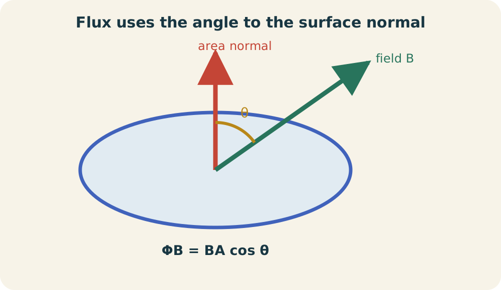
Magnetic flux measures how a magnetic field passes through an oriented surface. Its general definition is $\Phi_B=\int\mathbf B\boldsymbol\cdot d\mathbf A$. The Greek capital phi $\Phi_B$ denotes magnetic flux, and the subscript $B$ identifies the magnetic field. The vector area element $d\mathbf A$ points normal, or perpendicular, to each small piece of surface. The dot product keeps only the field component aligned with that normal.

For a uniform field through a flat area, the expression simplifies to $\Phi_B=BA\cos\theta$. The magnitude $B$ is measured in teslas, $A$ is measured in square meters, and $\theta$ is the angle between $\mathbf B$ and the chosen surface normal. The angle is not measured between the field and the plane of the loop. A field perpendicular to the plane is parallel to its normal and gives maximum flux magnitude. A field lying within the plane is perpendicular to the normal and gives zero flux.

Flux is measured in webers, abbreviated $\mathrm{Wb}$. One weber equals one tesla-square-meter, so $1\,\mathrm{Wb}=1\,\mathrm{T\,m^2}$. Flux is not magnetic-field strength and is not a count of physical field lines. Field-line drawings are visualization tools, while the flux integral is the quantitative definition. Changing area can change flux even when field strength stays fixed.

Orientation gives flux a sign

Every open surface used in a flux calculation has two possible normal directions. Choosing one direction as positive determines the sign of flux. A field component along the chosen normal contributes positive flux. A component opposite that normal contributes negative flux. Reversing the normal reverses every flux sign but does not change the underlying physics if the convention is used consistently.

For a wire loop, the right-hand rule connects positive circulation with positive surface normal. Curl the fingers of your right hand along the chosen positive path around the loop. Your thumb gives the associated positive normal. This convention becomes important when Faraday’s law is written with signs. Current and emf direction must use the same orientation pairing.

In many introductory problems, Lenz’s law can determine physical direction without a formal signed convention. Even then, it is useful to state whether flux into or out of the page is increasing or decreasing. Phrases such as “the field increases” are incomplete unless direction is included. An increasing negative flux and an increasing positive flux lead to different induced responses. Directional language is part of the calculation, not an optional illustration.

Four ways flux can change

The simplified expression $\Phi_B=BA\cos\theta$ reveals several mechanisms. Field magnitude $B$ can change while area and orientation remain fixed. Effective area $A$ can change as a loop expands, contracts, or enters a field region. Orientation angle $\theta$ can change as the loop rotates. More generally, a nonuniform field distribution can change across the surface.

A constant magnetic field can therefore produce changing flux. Rotating a loop changes the dot product even when $B$ is constant. Sliding an entire loop within an infinite uniform field without rotating or changing area does not change flux. Moving the loop across the edge of a finite field region changes the portion of area threaded by the field. The geometry of the field-loop system matters.

Conversely, a changing magnetic field does not guarantee nonzero flux through every loop. If the field always lies in the plane of a fixed flat loop, the dot product can remain zero. Symmetry can also make positive and negative contributions cancel across a more complicated surface. Induction depends on the change in net flux linkage. Field change and flux change must not be treated as synonyms.

Faraday’s law measures the rate of change

For one loop, Faraday’s law is $\mathcal E=-\frac{d\Phi_B}{dt}$. The script symbol $\mathcal E$ denotes electromotive force, commonly called emf, measured in volts. Despite its name, emf is not a force in newtons. It represents energy supplied per unit charge around a circuit. The derivative is the instantaneous rate at which signed flux changes.

For a tightly wound coil of $N$ identical turns, the model becomes $\mathcal E=-N\frac{d\Phi_B}{dt}$. The dimensionless integer $N$ counts turns that share approximately the same flux. The product $N\Phi_B$ is flux linkage. More turns produce greater emf magnitude for the same flux-change rate per turn. Coil geometry and field uniformity must support the identical-turn assumption.

Over a finite interval with approximately constant rate, the average emf is $\mathcal E_{\mathrm{avg}}=-N\frac{\Delta\Phi_B}{\Delta t}$. Webers per second equal volts. This unit identity can be written $1\,\mathrm{V}=1\,\frac{\mathrm{Wb}}{\mathrm{s}}$. Faster flux change produces larger emf magnitude. The total flux value matters less than how rapidly it changes during the interval.

Lenz’s law determines opposition

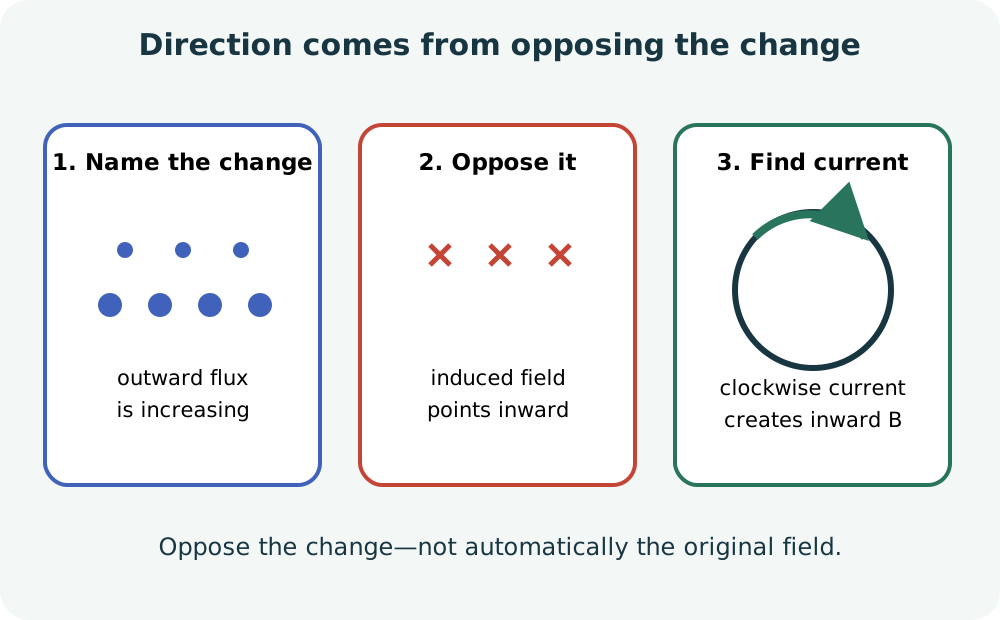
The minus sign in Faraday’s law encodes Lenz’s law. The induced current produces a magnetic field that opposes the change in magnetic flux. It does not necessarily oppose the original external field. If outward flux is increasing, the induced field points inward. If outward flux is decreasing, the induced field points outward to resist that decrease.

A reliable direction procedure has three steps. First state the direction of the original flux and whether its magnitude is increasing or decreasing. Second choose the induced field that opposes that change. Third use a loop right-hand rule to find the current direction that creates the induced field. Curling fingers along current makes the thumb point along the loop’s induced magnetic field.

Suppose a north pole approaches a loop along its axis. The external flux through the loop increases in the direction away from the approaching north pole. The loop creates an opposing field directed toward that pole. Its near face behaves like a north pole and repels the approaching magnet. Reversing the magnet’s motion reverses the current because the loop then tries to preserve the departing flux.

Energy conservation explains the minus sign

Imagine that an approaching magnet induced a loop field that strengthened the approach rather than opposing it. The magnet would accelerate toward the loop while induced current grew. The growing current could deliver thermal energy to a resistor without corresponding external work. Such positive feedback would create energy from nothing in the idealized account. Lenz’s-law opposition prevents that violation.

With the actual direction, an external agent must push against magnetic resistance to keep the magnet moving toward the loop. The agent does mechanical work. Energy is transferred into the circuit and can become internal energy in a resistor. Pulling the magnet away can also require work because the induced response resists the decrease in flux. Induction converts energy rather than generating it without a source.

The magnetic field participates in the interaction but should not be described as an inexhaustible fuel. A permanent magnet’s field helps organize forces, while the moving agent supplies energy in a simple generator demonstration. In other systems, a turbine, falling mass, chemical process, or changing current in another coil supplies the input. A complete explanation names the source, transfer pathway, and receiving account. Lenz’s law is then seen as an energy-consistent direction principle.

Worked changing-field example

A $50$-turn coil has area $0.0200\,\mathrm{m^2}$. Its surface normal is parallel to a uniform field that rises from $0.100\,\mathrm{T}$ to $0.400\,\mathrm{T}$ in $0.200\,\mathrm{s}$. Because $\theta=0$, the cosine factor is one. The flux change per turn is $\Delta\Phi_B=A\Delta B=(0.0200\,\mathrm{m^2})(0.300\,\mathrm{T})=6.00\times10^{-3}\,\mathrm{Wb}$. The sign depends on the chosen normal, while this value is the magnitude.

The average emf magnitude is $|\mathcal E|=N\frac{|\Delta\Phi_B|}{\Delta t}$. Substitution gives $|\mathcal E|=50\frac{6.00\times10^{-3}\,\mathrm{Wb}}{0.200\,\mathrm{s}}=1.50\,\mathrm{V}$. The weber-per-second unit becomes volts. A doubled time interval with the same total flux change would halve the average emf. A doubled turn count would double it.

To determine direction, suppose the increasing external field points into the page. The loop must create a field out of the page to oppose increasing inward flux. A right-hand rule shows that counterclockwise conventional current creates an outward field. The induced current is therefore counterclockwise when viewed from the page-facing side. If the circuit were open, the emf would remain but sustained conduction current would not flow.

Emf, current, and resistance are different

Faraday’s law predicts emf, not automatically current. If the conducting loop has total resistance $R$, an ohmic approximation gives $I=\frac{|\mathcal E|}{R}$ for current magnitude. The symbol $I$ is measured in amperes and $R$ in ohms. An open loop can have induced emf across its gap while current remains zero. Connectivity and impedance matter after induction establishes the electric drive.

In circuits with inductance or capacitance, current may not follow a simple instantaneous emf-over-resistance ratio. Changing current itself creates flux and self-induced emf. Alternating-current behavior can involve phase relationships. The basic Faraday principle still applies, but the circuit model must include all relevant elements. A calculation should not silently assume a purely resistive loop.

Current direction is determined after physical flux-change opposition is understood. The induced emf direction is the direction in which positive charge would be driven around the loop. Actual electron drift in a metal is opposite conventional current. This is the same convention used in ordinary circuit analysis. Mixing electron motion into the loop right-hand rule without care reverses conclusions.

Motional emf from magnetic force

Induction can also occur when a conductor moves through a magnetic field. Consider a rod of length $\ell$ moving with speed $v$ so that rod, velocity, and field are mutually perpendicular. Mobile charges experience magnetic force $q\mathbf v\times\mathbf B$. Positive and negative charges separate along the rod until an internal electric field balances further separation. The potential difference across the rod is a motional emf.

Under the ideal perpendicular geometry, the magnitude is $\mathcal E=B\ell v$. The symbol $\ell$ is rod length in meters, not the number one. Teslas times meters times meters per second reduces to volts. Faster motion, a longer rod, or a stronger field produces larger emf. For nonperpendicular geometry, only the appropriate cross-product component contributes.

Direction follows the magnetic-force rule for positive charge. Point right-hand fingers along rod velocity and curl toward the field. The thumb indicates which end becomes positive. Negative charges move oppositely. Once charge separation creates an electric force equal and opposite to magnetic force, a steady open-circuit potential difference can remain.

Sliding-rod generator and energy

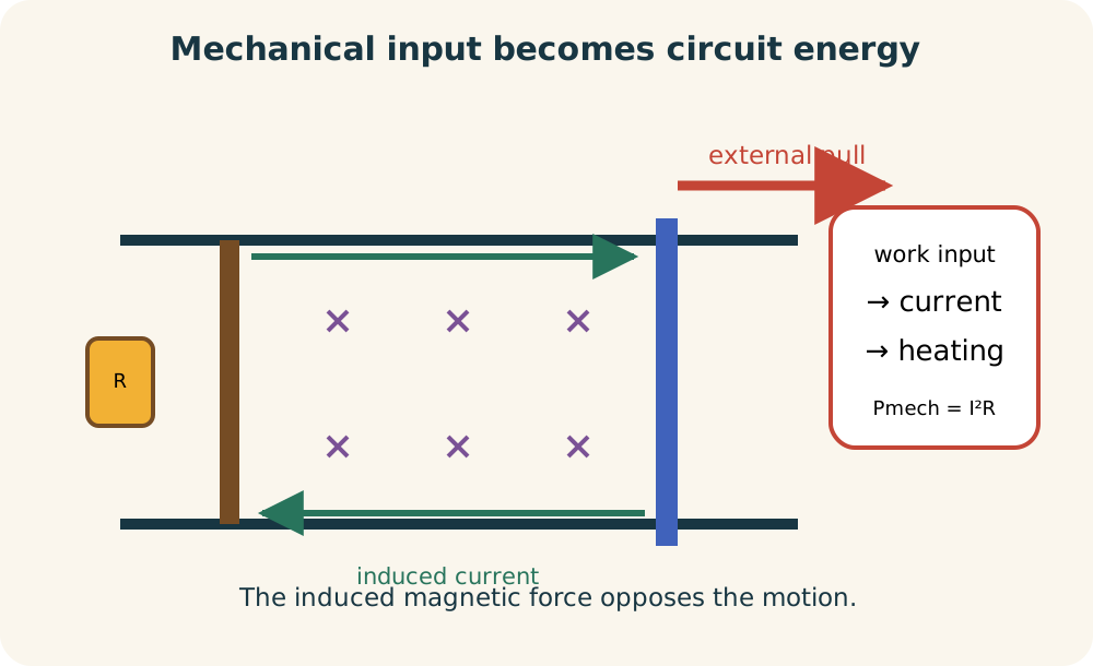
Place a conducting rod across parallel rails connected by a resistor, and move the rod through a uniform magnetic field. The rod and rails form a loop whose area changes. Faraday’s flux method and the motional-force method give the same emf magnitude $B\ell v$. If the total resistance is $R$, current magnitude is $I=\frac{B\ell v}{R}$. The current creates a magnetic force on the rod opposing its motion.

An external agent must pull with equal force to maintain constant speed. The magnetic force magnitude on the rod is $F_B=I\ell B$ under perpendicular conditions. Mechanical input power is $P_{\mathrm{mech}}=F_Bv$. Substituting current gives $P_{\mathrm{mech}}=\frac{B^2\ell^2v^2}{R}$. Electrical thermal power is $P_{mathrm{thermal}}=I^2R$, which gives the same expression.

This equality displays energy conservation explicitly. Mechanical work done by the agent becomes electrical energy and then internal energy in the resistor under the ideal model. If the agent stops pulling, the opposing magnetic force slows the rod. The rod’s kinetic energy can then supply a temporary current and heating. Lenz’s-law direction ensures the mechanical and electrical accounts remain consistent.

Rotating loops and generators

A loop rotating in a uniform magnetic field has time-varying orientation. If its normal rotates at angular speed $\omega$, an ideal flux can be written $\Phi_B=BA\cos(\omega t)$. The argument $\omega t$ is the angle in radians between field and normal. Differentiating gives an emf proportional to $\sin(\omega t)$. The induced emf alternates direction periodically.

For $N$ turns, the ideal emf is $\mathcal E=NBA\omega\sin(\omega t)$ after a suitable orientation convention. Its maximum magnitude is $\mathcal E_{max}=NBA\omega$. Increasing turn count, field strength, loop area, or rotation rate raises the ideal peak. Real generators include magnetic circuits, winding geometry, internal resistance, and losses. The simple formula reveals the foundational dependencies.

A generator converts mechanical input into electrical output. A turbine driven by moving water, steam, wind, or an engine provides torque. Magnetic interactions oppose motion when current supplies a load, so maintaining speed requires continued input work. Removing the electrical load reduces the required mechanical torque under comparable conditions. Generation is an energy-conversion process governed by induction and conservation.

Mutual induction and transformers

A changing current in one coil creates a changing magnetic field. If some of that field threads a second coil, the second coil experiences changing flux and induced emf. This process is mutual induction. The coils need not touch electrically. Their coupling occurs through the electromagnetic field.

An ideal transformer uses alternating current in a primary coil to create changing magnetic flux through a core and secondary coil. The voltage ratio is approximately $\frac{V_s}{V_p}=\frac{N_s}{N_p}$ in an ideal tightly coupled model. Subscripts $p$ and $s$ label primary and secondary quantities. A larger secondary turn count gives a higher secondary voltage. Ideal power conservation implies a corresponding current tradeoff.

A transformer does not operate indefinitely from steady direct current. After a DC switching transient, current and flux may become constant, leaving no continuing secondary emf. Alternation keeps flux changing. Real transformers have winding resistance, leakage flux, eddy currents, and core hysteresis. Faraday’s law supplies the foundation while engineering models account for losses.

Eddy currents and magnetic braking

Changing flux through bulk conductors can drive circulating currents called eddy currents. Those currents create magnetic fields that oppose the changes producing them. They can generate drag on moving conductors. The drag transfers mechanical energy into internal energy. Magnetic braking can therefore operate without ordinary surface friction at the braking interface.

Eddy currents are useful in induction heating, damping instruments, and braking systems. They can also waste energy in transformer cores and motors. Laminating a conducting core interrupts large current loops and reduces eddy-current losses. Material resistivity and geometry influence their strength. The same phenomenon can be either desired or undesirable depending on system purpose.

Dropping a magnet through a conducting tube provides a striking demonstration. Changing flux induces currents in the tube walls. Their magnetic interaction opposes the magnet’s fall, so it descends more slowly than in a nonconducting tube. Gravitational potential energy becomes internal energy in the tube and surroundings. No contact friction is required for the energy transfer.

Common reasoning failures

One error treats flux as simply $BA$ without checking orientation. The correct uniform-field expression includes $\cos\theta$ with angle measured from the surface normal. A field lying in the loop’s plane produces zero flux through that flat surface. Draw the normal before choosing the angle. This single step prevents the common complementary-angle mistake.

Another error says induced current opposes the magnetic field. Lenz’s law says it opposes the change in magnetic flux. When an outward field decreases, the induced field is also outward because it resists the decrease. When the outward field increases, the induced field points inward. Naming both direction and change resolves the apparent contradiction.

A third error obtains emf and assumes current without checking the circuit. An open loop can support induced potential difference but not a sustained circulating current. A closed loop’s current depends on resistance and possibly inductance or capacitance. Another error omits the external energy source in a generator. The required mechanical work explains the electrical output and Lenz-law opposition.

Practice and retrieval

A flat loop of area $0.500\,\mathrm{m^2}$ lies with its normal parallel to a $0.200\,\mathrm{T}$ field. Calculate flux with units. Then rotate the loop until its plane is parallel to the field and calculate the new flux. State the angle used in each case. Explain why the second wording corresponds to maximum rather than zero flux.

A $200$-turn coil experiences a flux-per-turn change from $+4.00\times10^{-4}\,\mathrm{Wb}$ to $-1.00\times10^{-4}\,\mathrm{Wb}$ in $0.0500\,\mathrm{s}$. Calculate average emf magnitude. Explain what the signs mean relative to the selected normal. State how the induced direction would be determined. Predict the effect of doubling the time interval.

A $0.400\,\mathrm{m}$ rod moves at $6.00\,\frac{\mathrm{m}}{\mathrm{s}}$ perpendicular to a $0.750\,\mathrm{T}$ field. Calculate motional emf. If the complete loop resistance is $3.00\,\Omega$, calculate current and thermal power. Identify the external energy source when the rod maintains constant speed. Explain why induced magnetic force opposes motion.

Solutions and reasoning

Initially $\theta=0$, so $\Phi_B=BA=(0.200\,\mathrm{T})(0.500\,\mathrm{m^2})=0.100\,\mathrm{Wb}$. When the plane is parallel to the field, its normal is perpendicular to the field and $\theta=90^\circ$. The new flux is zero. If the plane were perpendicular to the field, its normal would be parallel and flux would be maximum. Surface-normal language resolves the wording.

The signed change is $\Delta\Phi_B=-1.00\times10^{-4}-4.00\times10^{-4}=-5.00\times10^{-4}\,\mathrm{Wb}$ per turn. Emf magnitude is $|\mathcal E|=N\frac{|\Delta\Phi_B|}{\Delta t}=200\frac{5.00\times10^{-4}\,\mathrm{Wb}}{0.0500\,\mathrm{s}}=2.00\,\mathrm{V}$. Signs record flux relative to the chosen normal. Lenz’s law and a right-hand rule determine current direction. Doubling time for the same flux change halves average emf.

Motional emf is $\mathcal E=B\ell v=(0.750\,\mathrm{T})(0.400\,\mathrm{m})(6.00\,\frac{\mathrm{m}}{\mathrm{s}})=1.80\,\mathrm{V}$. Current is $I=\frac{1.80\,\mathrm{V}}{3.00\,\Omega}=0.600\,\mathrm{A}$. Thermal power is $P=I^2R=(0.600\,\mathrm{A})^2(3.00\,\Omega)=1.08\,\mathrm{W}$. An external agent supplies mechanical energy while maintaining speed. The opposing magnetic force makes that energy account consistent with Lenz’s law.

Connection forward

Induced emf enters circuit equations like other emf sources, but its origin lies in changing flux. Kirchhoff’s rules can then determine currents and voltage changes in connected networks. When current changes create self-induced emf, inductors store energy in magnetic fields. Differential equations describe the resulting transients. Induction therefore bridges field reasoning and circuit dynamics.

Faraday’s law also points beyond circuit loops. A changing magnetic field is associated with a circulating electric field even when no conducting wire is present. This broader statement is one of Maxwell’s equations. Together with the magnetic field created by changing electric conditions, it supports electromagnetic waves. The loop experiment reveals a foundational field relationship.

Carry forward four questions. What surface and normal define flux, what feature changes, what induced field opposes that change, and where does the transferred energy originate? Use Faraday’s law for magnitude and Lenz’s law for direction. Check whether the circuit is open or closed before claiming current. With these habits, induction becomes a coherent energy-and-field model rather than a collection of hand rules.