Confidence Intervals

A sample gives one estimate, but another random sample would usually give a different value. A confidence interval uses that sample-to-sample variability to report a range of parameter values compatible with the data and method. The interval is not a decorative plus-or-minus attached to an estimate. Its reliability depends on sampling design, model conditions, standard-error calculation, and repeated-sampling behavior. Learning to interpret that behavior prevents one of the most common errors in introductory statistics.

Learning objectives and the central inference question

By the end of this lesson, you will distinguish parameters from statistics and explain why sampling distributions make interval estimation possible. You will build intervals in estimate-plus-or-minus-margin form, calculate standard errors, and choose appropriate critical values. You will check conditions for one-proportion and one-mean procedures. You will interpret confidence level and realized intervals accurately. You will also analyze width, sample size, bias, practical importance, and sources of error beyond sampling.

The central inference question asks how much this estimate would vary if the sampling process were repeated. The observed sample cannot display that repeated variability by itself. Probability models and sampling theory describe the distribution of an estimator across hypothetical repetitions. Its spread determines how precisely the sample locates the population parameter. Confidence intervals convert that estimated spread into an interpretable range. Repetition is conceptual even when only one real sample is collected.

Inference always links data to a target. State the population, parameter, sample, and statistic before computing. A population proportion $p$ is fixed but unknown, while a sample proportion $\hat p$ changes from sample to sample. A population mean $\mu$ is fixed but unknown, while a sample mean $\bar x$ varies. Notation keeps the target separate from the evidence used to estimate it.

Distinguish parameters, statistics, and estimators

A parameter is a numerical feature of a population or probability model. Examples include population mean $\mu$, population proportion $p$, and population standard deviation $\sigma$. Parameters are typically fixed within a frequentist analysis, even though their values are unknown. A statistic is calculated from sample data. It is observable after the sample is collected.

An estimator is a rule for calculating a statistic intended to approximate a parameter. The sample mean $\bar X$ is an estimator of $\mu$, while its realized value $\bar x$ is the estimate from one sample. Uppercase notation sometimes emphasizes the random estimator before data are observed. Lowercase notation records the observed outcome. Courses differ in typography, so the conceptual distinction matters more than capitalization.

Estimator quality has several dimensions. Bias describes systematic displacement of the estimator’s sampling center from the target. Variability describes how much estimates differ across samples. A low-variability estimator can still be badly biased, and a centered estimator can still be imprecise. Confidence procedures need both an appropriate center and a dependable spread estimate.

Build a sampling distribution through repetition

Imagine repeatedly drawing random samples of the same size from one population and calculating the same statistic each time. The distribution of those statistic values is the sampling distribution. It has a center, spread, and shape just as a distribution of individual observations does. However, its observational units are estimates rather than individual cases. Confusing these two distributions leads to incorrect standard errors.

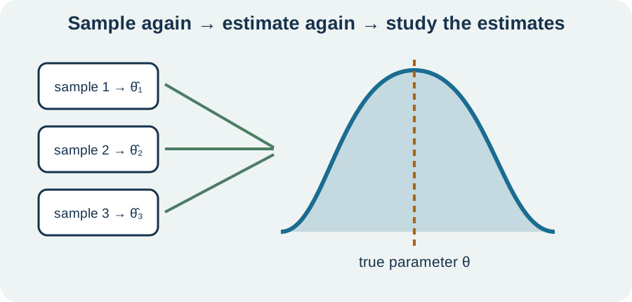
For an unbiased estimator, the sampling distribution is centered at the true parameter. Its standard deviation is called the standard error when known or estimated from data according to common usage. Smaller standard error means estimates cluster more tightly around the parameter. Larger samples usually reduce this spread. The exact rate depends on the estimator and sampling design.

The shape matters because critical values describe central regions of a reference distribution. Normal and $t$ approximations work when stated conditions make the standardized estimator behave accordingly. Strong skewness, small samples, dependence, or boundary proportions can defeat simple approximations. A formula is valid only within its inferential framework. Conditions connect the observed study to the reference distribution.

Separate observation spread from estimator uncertainty

The sample standard deviation $s$ describes spread among individual measured values. The standard error of the sample mean estimates spread among means from repeated samples. For independent observations, $\operatorname{SE}(\bar x)=\frac{s}{\sqrt n}$. The horizontal fraction divides individual spread by the square root of sample size. Averaging reduces sampling variability because positive and negative individual deviations partly balance.

Suppose measurements have sample standard deviation $12\ \mathrm{mg}$ and sample size $n=36$. The estimated standard error is $\frac{12\ \mathrm{mg}}{\sqrt{36}}=2.0\ \mathrm{mg}$. Individual measurements vary on a roughly twelve-milligram scale, while sample means vary on a roughly two-milligram scale. Both quantities retain response units. They answer different questions.

For a sample proportion, a common estimated standard error is $\operatorname{SE}(\hat p)=\sqrt{\frac{\hat p(1-\hat p)}{n}}$. The expression $1-\hat p$ is the sample proportion outside the category. Proportions are dimensionless, so their standard errors are dimensionless. The square root restores the scale after multiplying and dividing variance components. Boundary values near zero or one require particular care with normal approximations.

Derive estimate plus or minus margin of error

Many confidence intervals have the form estimate plus or minus critical value times standard error. Symbolically, write $\hat\theta\pm c^*\operatorname{SE}(\hat\theta)$. The symbol $\hat\theta$ stands for a general estimator, and $c^*$ is a critical value from a reference distribution. The product $c^*\operatorname{SE}$ is the margin of error. Subtracting and adding it produces lower and upper endpoints.

The critical value determines how much standardized sampling probability is included. For a central $95\%$ normal interval, $z^*\approx1.96$. Approximately $95\%$ of a standard normal distribution lies between $-1.96$ and $1.96$. Higher confidence requires a wider central region and a larger critical value. The data do not determine the confidence level after the fact; it is part of the procedure.

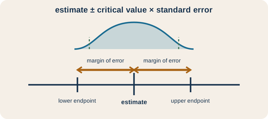
The margin of error measures sampling precision under the chosen method. It does not include every source of uncertainty automatically. Coverage bias, nonresponse, measurement error, model misspecification, and data processing can remain outside the formula. A narrow interval can be precisely wrong when the data are systematically biased. Design quality and interval width must be evaluated separately.

Construct a one-proportion interval

Suppose a random sample contains $x$ successes among $n$ eligible observations. The sample proportion is $\hat p=\frac{x}{n}$. A common large-sample interval is $\hat p\pm z^*\sqrt{\frac{\hat p(1-\hat p)}{n}}$. Every term is dimensionless. The interval estimates the corresponding population proportion $p$.

Before using this approximation, check the sampling design and success-failure counts. A common condition requires at least ten expected or observed successes and ten failures for the plug-in interval, depending on course convention. Random sampling or random assignment supports the probabilistic mechanism. When sampling without replacement, $n$ should commonly be no more than $10\%$ of the population to approximate independence. State rather than merely imply these conditions.

If $180$ of $300$ randomly sampled voters support a proposal, then $\hat p=\frac{180}{300}=0.600$. The estimated standard error is $\sqrt{\frac{(0.600)(0.400)}{300}}\approx0.0283$. With $z^*=1.96$, margin of error is approximately $(1.96)(0.0283)=0.0554$. The $95\%$ interval is approximately $(0.545,0.655)$, or $54.5\%$ to $65.5\%$. The endpoints describe plausible values for the population support proportion under the procedure.

Construct a one-mean t interval

For a population mean with unknown population standard deviation, use $\bar x\pm t^*\frac{s}{\sqrt n}$ under appropriate conditions. The critical value comes from a $t$ distribution with $n-1$ degrees of freedom for a one-sample mean. Degrees of freedom reflect how estimating the mean constrains deviations. The $t$ distribution has heavier tails than the standard normal distribution. Its critical values approach normal critical values as sample size grows.

Suppose a random sample of $64$ measurements has mean $12.4\ \mathrm{mg}$ and standard deviation $3.2\ \mathrm{mg}$. The standard error is $\frac{3.2\ \mathrm{mg}}{\sqrt{64}}=0.40\ \mathrm{mg}$. If the appropriate critical value is approximately $2.00$, margin of error is $0.80\ \mathrm{mg}$. The interval is $12.4\ \mathrm{mg}\pm0.80\ \mathrm{mg}$. Its endpoints are $11.6\ \mathrm{mg}$ and $13.2\ \mathrm{mg}$.

Mean-procedure robustness depends on sample size and population shape. With small samples, strong skewness or outliers can make the $t$ interval unreliable. Larger independent samples benefit from central-limit behavior, though severe pathologies still deserve attention. A plot of sample values can reveal outliers and shape concerns. The interval formula should follow, not replace, data inspection.

Interpret confidence through long-run coverage

A $95\%$ confidence procedure is designed so that about $95\%$ of intervals from repeated samples cover the fixed true parameter under the method’s assumptions. The intervals vary because the samples vary. The parameter does not jump among them. Some realized intervals miss. The confidence level describes the procedure’s long-run success rate.

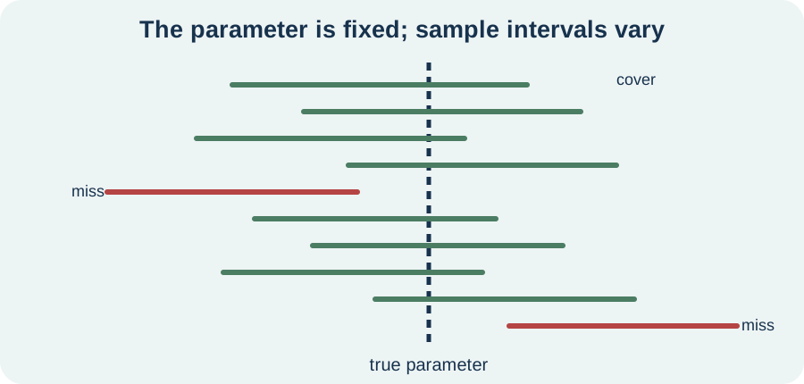
After one interval is calculated, it either covers the parameter or it does not. In ordinary frequentist interpretation, it is incorrect to assign $95\%$ probability to the fixed parameter lying inside that already observed interval. Before sampling, the random endpoints have a $95\%$ coverage probability. After sampling, their values are fixed. This timing distinction explains the conventional interpretation.

A contextual statement may say that we are $95\%$ confident the population mean lies between $11.6\ \mathrm{mg}$ and $13.2\ \mathrm{mg}$. The word confident refers to using a procedure with validated coverage behavior. Name the population parameter rather than saying vaguely that the data lie in the interval. Individual observations are not expected to fall inside a mean interval. The interval estimates a parameter, not the spread of raw data. Context should identify which population the mean describes.

Check randomization, independence, and shape

Randomization supplies a basis for probability calculations. A random sample supports inference to the population from which it was selected, while random assignment supports causal comparison in an experiment. Convenience samples may produce precise-looking intervals without representative coverage. The formula cannot create randomness after data collection. Study design determines the scope of inference.

Independence means one sampled outcome does not reveal or determine another in the way the method forbids. Sampling without replacement creates mild dependence, but the $10\%$ condition makes it negligible for many introductory procedures. Clustered, paired, repeated, or time-series data require methods that represent their dependence. Treating dependent observations as independent usually understates uncertainty. The effective information can be much smaller than the row count.

Distributional conditions depend on the estimator. Proportion methods need enough successes and failures for a normal approximation. Mean methods need an approximately normal population for small samples or enough independent data for robust sampling behavior. A histogram, boxplot, and context help evaluate shape. Conditions should be connected to evidence, not recited as a ritual.

Analyze confidence level and interval width

Holding data and method fixed, higher confidence produces a wider interval. A $99\%$ method must include more of the reference distribution than a $90\%$ method. Its critical value is therefore larger. Greater long-run coverage comes at the cost of lower precision. Confidence and width cannot both be improved merely by changing the label.

Holding confidence fixed, larger sample size usually narrows the interval. For many estimators, standard error is proportional to $\frac{1}{\sqrt n}$. Multiplying sample size by four halves the standard error and approximately halves the margin of error. Multiplying sample size by nine reduces standard error to one third. Precision improves with diminishing returns.

Holding sample size and confidence fixed, greater population variability produces a wider mean interval. Proportion standard error is largest near $p=0.5$ for fixed $n$. Better measurement can reduce variability unrelated to the target, while better design can avoid unnecessary dependence. Width is shaped by confidence, sample size, and variability. Interpreting it requires knowing which factor changed.

Plan sample size for a target margin

For a proportion using anticipated value $p^*$ and normal critical value $z^*$, target margin $M$ satisfies approximately $M=z^*\sqrt{\frac{p^*(1-p^*)}{n}}$. Solving gives $n=\frac{(z^*)^2p^*(1-p^*)}{M^2}$. Round the result upward because a smaller integer would miss the desired precision. The planned sample size may need adjustment for nonresponse or finite-population design. Planning assumptions should be documented.

If no prior proportion estimate is available, using $p^*=0.5$ is conservative because it maximizes $p(1-p)$. For $95\%$ confidence and target margin $0.03$, the calculation is $n=\frac{(1.96)^2(0.5)(0.5)}{(0.03)^2}\approx1067.1$. Rounding upward gives $1{,}068$ completed responses. If response rate is expected to be $60\%$, more people must be contacted. Completed sample and recruited sample are different planning quantities.

For a mean, planning requires an estimate of population standard deviation or a defensible pilot value. A rough normal formula is $n=\left(\frac{z^*\sigma}{M}\right)^2$. Unknown variability makes the plan uncertain. Sensitivity calculations across plausible standard deviations are more honest than one unsupported number. Ethical and resource constraints also shape feasible precision.

Separate precision from accuracy and bias

Precision describes how tightly repeated estimates cluster, while accuracy concerns closeness to the target. Increasing sample size reduces random sampling variability under the design. It does not automatically remove selection bias, measurement bias, or confounding. A huge biased sample can produce a very narrow interval centered at the wrong value. Narrowness alone is not evidence of validity.

Nonresponse can bias a survey when respondents differ systematically from nonrespondents on the target. Calibration error can shift every measurement. Coverage error can exclude parts of the population. Processing rules can introduce misclassification. Ordinary confidence intervals usually account for none of these unless the model explicitly represents them.

Ask what uncertainty is included in the standard error. Complex surveys may require weights, strata, clusters, or replicate methods. Laboratory measurements may require calibration and propagation of instrument uncertainty. Model-based intervals depend on model assumptions. The phrase “margin of error” should not be advertised as total error without justification.

Connect intervals with hypothesis tests

Confidence intervals and two-sided hypothesis tests often use the same standardized sampling machinery. At matching levels, a $95\%$ interval commonly excludes exactly those null values rejected by a two-sided test at significance level $0.05$. The interval shows a range of compatible parameter values, while the test evaluates one specified value. Both depend on the same conditions. Neither measures practical importance automatically.

If a difference interval excludes zero, the corresponding null of no difference may be rejected at the matched level. The distance from zero and endpoint magnitudes also communicate effect size and precision. A tiny effect can be statistically detectable in a very large sample. A practically important effect can remain uncertain in a small sample. Decisions require context beyond inclusion or exclusion.

One-sided tests correspond to one-sided confidence bounds rather than ordinary two-sided intervals. Post hoc switching between one-sided and two-sided procedures changes error rates. Choose the inferential question before examining results. Multiple intervals and repeated analyses also affect collective coverage. A single-interval confidence level does not describe an entire exploratory workflow.

Diagnose common interpretation mistakes

Do not say that $95\%$ of population values lie inside a confidence interval for the mean. The interval targets the population mean, while raw observations have their own distribution. A prediction interval for a future observation is usually wider. Different intervals target different random quantities. Name the target explicitly.

Do not say the procedure guarantees this particular interval contains the parameter. Coverage is a long-run frequency under assumptions. Nor should confidence level be interpreted as the fraction of the sample lying inside the endpoints. The sample may contain many values outside a mean interval. Confidence concerns parameter estimation.

Do not use confidence intervals to hide design failures. If data are not representative or assumptions are contradicted, numerical endpoints can be misleading. Report violations and use an appropriate alternative when possible. A mechanically correct calculation is not necessarily valid inference. Conditions and interpretation are part of the answer.

Verify an interval in a reproducible sequence

Begin by identifying the population, parameter, sample, statistic, and intended confidence level. Name the procedure and state its formula. Check randomization, independence, and distributional conditions with evidence. Confirm the data type matches the procedure. Do not choose the method solely from which formula is familiar.

Next calculate the point estimate, standard error, critical value, margin of error, and endpoints with units. Keep extra precision until the final step. Verify that the estimate is the midpoint of a symmetric interval when the method has that form. For proportions, check whether endpoints remain plausible and consider improved methods near boundaries. For means, inspect the sample distribution.

Finally write a contextual interpretation and a limitations statement. Name the fixed parameter and repeated-sampling confidence procedure. Explain the scope supported by sampling or assignment. Distinguish sampling uncertainty from other errors. A complete interval analysis is a chain of reasoning, not two numbers in parentheses.

Practice calculation, planning, and interpretation

A random sample of $64$ measurements has mean $12.4\ \mathrm{mg}$ and standard deviation $3.2\ \mathrm{mg}$. Using $t^*=2.00$, calculate standard error, margin of error, and interval endpoints. State a correct contextual interpretation. Explain which evidence you would inspect before trusting the $t$ procedure. Distinguish individual measurement spread from mean uncertainty.

A poll reports $600$ supporters among $1{,}000$ randomly sampled eligible voters. Construct an approximate $95\%$ one-proportion interval using $z^*=1.96$. Check the success-failure condition. Interpret the interval without assigning probability to the fixed population proportion after sampling. Explain what nonresponse bias could do despite the large sample. Report endpoints as percentages.

Plan a $95\%$ proportion interval with margin of error at most $0.02$ when no prior proportion is available. Use the conservative value $p^*=0.5$. Calculate and round sample size correctly. Then explain how the requirement changes if the target margin is halved. State why quadrupling appears. Separate completed responses from contacts required under nonresponse.

Solutions and reasoning

For the mean, standard error is $\frac{3.2\ \mathrm{mg}}{\sqrt{64}}=0.40\ \mathrm{mg}$. Margin of error is $(2.00)(0.40\ \mathrm{mg})=0.80\ \mathrm{mg}$. The interval is $(11.6\ \mathrm{mg},13.2\ \mathrm{mg})$. A correct interpretation refers to confidence in the procedure estimating the population mean. Sample design, independence, outliers, and distribution shape must be checked.

For the poll, $\hat p=0.600$ and standard error is $\sqrt{\frac{(0.600)(0.400)}{1000}}\approx0.01549$. Margin of error is approximately $(1.96)(0.01549)=0.0304$. The interval is approximately $(0.570,0.630)$, or $57.0\%$ to $63.0\%$. Counts of $600$ successes and $400$ failures easily satisfy the large-count condition. Nonresponse can shift the interval away from the population value without making it visibly wider.

For planning, $n=\frac{(1.96)^2(0.5)(0.5)}{(0.02)^2}=2401$. This value is already an integer, so $2{,}401$ completed responses are required under the approximation. Halving the target margin to $0.01$ multiplies required sample size by four because $n$ is inversely proportional to $M^2$. If only a fraction respond, more contacts are needed. Planning should include expected response rate and design effects.

Carry interval reasoning into later inference

Confidence intervals connect sampling design, probability, estimation, and communication. Their center comes from a statistic, their width comes from sampling uncertainty and confidence level, and their validity comes from conditions. No component can be interpreted in isolation. A narrow interval from poor data is not a trustworthy answer. A wide interval honestly reports limited information.

Hypothesis testing uses the same standardized estimators and reference distributions to evaluate specified parameter values. Regression extends intervals to slopes, mean responses, and predictions. Bootstrap procedures approximate sampling distributions through resampling. Bayesian intervals use a different probability interpretation based on a posterior distribution. Knowing which framework generated an interval is essential.

When presenting an interval, state the target, population, confidence level, endpoints, units, method, and principal limitations. Explain confidence through repeated-sampling coverage. Separate sampling precision from total accuracy. That discipline turns interval notation into a transparent claim about what the data can and cannot establish. Good reporting keeps uncertainty visible instead of burying it behind an estimate.