Hypothesis Testing

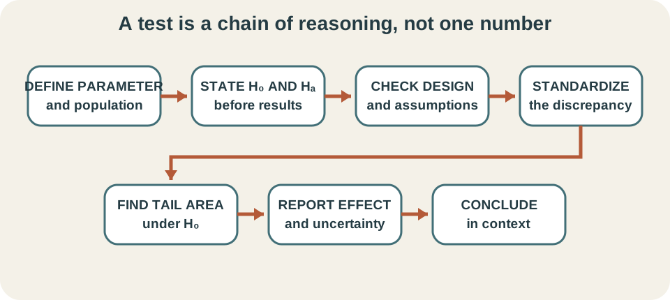
A hypothesis test asks how surprising the observed data would be if a specified null model and its assumptions were true. It does not calculate the probability that the null hypothesis is true, nor does it replace scientific judgment with a threshold. A complete test begins with a parameter and study design, moves through a reference distribution, and ends with a calibrated interpretation. Effect size, uncertainty, assumptions, and practical consequences remain essential after the p-value is computed. This lesson builds that complete chain of reasoning.

Establish the learning goals

By the end of this lesson, you should be able to formulate null and alternative hypotheses about a population parameter. You will explain how a test statistic measures discrepancy in standard-error units. You will define and interpret a p-value without reversing its conditional probability. You will distinguish Type I error, Type II error, significance level, and power. You will also connect tests with confidence intervals and report practical importance alongside statistical evidence.

The aim is not to memorize a catalogue of named procedures. Most familiar tests share the same logical structure: compare an estimate with a null value, standardize the difference, and evaluate it under a reference model. What changes from problem to problem is the parameter, estimator, standard error, assumptions, and direction of the alternative. Understanding that structure makes procedures easier to select and critique. It also prevents software output from becoming a substitute for reasoning.

Every test should answer four questions. What population parameter or model is being evaluated? What would the data-generating process look like if the null were true? Which discrepancies count as evidence for the stated alternative? What consequences follow from acting on the result? These questions keep inference tied to both probability and context.

Define the parameter before the hypotheses

A hypothesis concerns a population parameter or data-generating model, not the numerical statistic already observed. A population mean is commonly written $\mu$, a population proportion is written $p$, and a population regression slope may be written $\beta_1$. Sample counterparts such as $\overline x$, $\widehat p$, and $b_1$ estimate those parameters. The distinction matters because inferential uncertainty arises from using a sample to learn about a population. A hypothesis should name the unknown target explicitly.

The target population must also be stated. Testing a mean for “students” is ambiguous unless the school, grade, time, and sampling frame are identified. Generalization depends on how observations entered the sample. Random sampling supports population inference when nonresponse and coverage problems are controlled. Convenience sampling can still describe the observed cases but weakens broader claims.

Units belong in parameter statements when the parameter measures a physical quantity. If a filling process targets a mean mass of $50.0\,\mathrm{grams}$, then $\mu$ is measured in grams. If a parameter is a proportion, it is dimensionless but should still be tied to a clearly defined outcome. If two means are compared, their difference retains the response unit. Precise definitions make the hypotheses interpretable before any arithmetic begins.

Formulate null and alternative hypotheses

The null hypothesis, written $H_0$, specifies a reference value or model. A two-sided mean test might use $H_0:\mu=50.0\,\mathrm{grams}$. The alternative hypothesis, written $H_A$ or $H_1$, describes departures that would answer the research question, such as $H_A:\mu\ne50.0\,\mathrm{grams}$. The symbol $\ne$ indicates deviations in either direction. Both statements concern the same population parameter.

A one-sided alternative uses a direction established before results are examined. For example, $H_A:\mu>50.0\,\mathrm{grams}$ treats only larger means as evidence against the null in the chosen test. Data far below the target would not support that alternative, even if they are surprising under the null. Choosing direction after observing the estimate unfairly reduces the reported p-value. Direction must come from the scientific or decision question.

The null is often an equality because an exact reference value determines a sampling distribution for the test statistic. This convention does not mean the analyst believes the value is literally perfect. It supplies a benchmark against which discrepancy is measured. In equivalence or noninferiority studies, the hypothesis structure may be reversed or use a margin rather than a point. The hypotheses must match the claim the study is designed to support.

Build a standardized test statistic

A common test statistic has the form $\frac{\text{estimate}-\text{null value}}{\text{standard error under }H_0}$. The numerator measures raw discrepancy in the parameter’s unit. The denominator estimates how much the statistic would vary from sample to sample under the null model. Dividing cancels the unit and expresses discrepancy in standard-error units. Larger absolute values indicate estimates farther from the null relative to expected sampling noise.

For a one-sample mean with unknown population standard deviation, the statistic is $t=\frac{\overline x-\mu_0}{s/\sqrt n}$. Here $\overline x$ is the sample mean, $\mu_0$ is the null mean, $s$ is the sample standard deviation, and $n$ is sample size. The quantity $s/\sqrt n$ is the estimated standard error of the sample mean. Both the numerator and denominator have response units. Their ratio $t$ is dimensionless.

Standardization makes evidence depend on both effect magnitude and precision. A one-gram difference can be weak evidence in a noisy small sample but strong evidence in a stable large sample. This is why a p-value does not directly measure effect size. It combines discrepancy with sampling uncertainty. Report the estimate in original units so readers can separate those ideas.

Construct the null reference distribution

The reference distribution describes how the test statistic would behave over repeated samples if $H_0$ and the procedure’s assumptions were true. For the one-sample mean statistic with normally distributed observations, the reference distribution is a Student $t$ distribution with $n-1$ degrees of freedom. The degrees of freedom reflect estimating the population standard deviation from the same sample. As degrees of freedom increase, the $t$ distribution approaches the standard normal distribution. The distribution translates standardized discrepancy into tail probability.

Reference distributions can be theoretical, simulated, permuted, or bootstrapped. A randomization test may repeatedly reassign treatment labels according to the original randomization design. A simulation under a binomial null may generate many samples using the hypothesized success probability. The method must reproduce the null mechanism relevant to the study. Merely shuffling data without respecting groups, pairing, or dependence can produce the wrong reference distribution.

Assumptions connect the observed study to the reference calculation. Independence may follow from design or require modeling. Normal approximations require adequate sample size and distributional conditions. A paired test requires meaningful within-pair differences rather than independent-group analysis. Checking assumptions is part of computing evidence, not an optional afterthought.

Interpret the p-value correctly

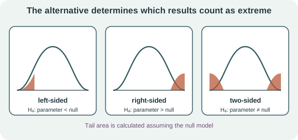
The p-value is the probability, assuming the null model and required assumptions, of obtaining a test statistic at least as extreme as the observed statistic in the direction specified by the alternative. The phrase “assuming the null” is essential. The p-value is a probability about possible data or statistics under a model. It is not the probability that the null itself is true. Reversing those conditional statements is a serious logical error.

For a two-sided alternative, extremeness usually includes both tails of a symmetric reference distribution. For a right-sided alternative, only sufficiently large statistics count. For a left-sided alternative, only sufficiently small statistics count. The observed direction and the predeclared alternative therefore determine the tail area. A two-sided p-value is not chosen merely because it is larger or smaller.

Suppose a valid analysis yields $p=0.03$. A correct interpretation is that, if the null model and assumptions were true, results at least as extreme in the specified sense would occur with probability $0.03$. It does not mean there is a three-percent probability that the null is true. It also does not mean the result has a ninety-seven-percent chance of replicating. Those claims require different models and information.

Work through a one-sample mean test

A filling process targets $50.0\,\mathrm{grams}$. A random sample of $25$ items has mean $\overline x=51.2\,\mathrm{grams}$ and standard deviation $s=3.0\,\mathrm{grams}$. Consider $H_0:\mu=50.0\,\mathrm{grams}$ against $H_A:\mu\ne50.0\,\mathrm{grams}$. The estimated standard error is $\frac{3.0\,\mathrm{grams}}{\sqrt{25}}=0.60\,\mathrm{grams}$. The observed mean is two standard errors above the null value.

The test statistic is $t=\frac{51.2\,\mathrm{grams}-50.0\,\mathrm{grams}}{0.60\,\mathrm{grams}}=2.00$. Gram units cancel, leaving a dimensionless statistic. Under the null and assumptions, this statistic follows a $t$ distribution with $25-1=24$ degrees of freedom. A two-sided p-value includes values at least as far from zero in both directions. Software or a table gives a value a little above $0.05$.

The calculation alone is not the conclusion. The sample should be examined for independence, severe skew, and influential observations, especially because the procedure estimates uncertainty from only twenty-five values. The estimated mean difference is $1.2\,\mathrm{grams}$, whose practical importance depends on production tolerances and consequences. A confidence interval communicates the range of mean differences compatible with the same data and assumptions. Evidence, magnitude, and decision consequences should be reported together.

Use decision rules without turning off judgment

A significance level $\alpha$ is a long-run Type I error rate selected before examining results. A common convention is $\alpha=0.05$, but no universal law makes five percent appropriate for every decision. Under a valid continuous test, rejecting when $p\le\alpha$ controls the probability of rejection at no more than $\alpha$ when the null is true. The threshold defines a procedure over repeated studies. It is not the probability that this particular rejection is wrong.

If $p\le\alpha$, the formal language is “reject $H_0$.” If $p>\alpha$, use “fail to reject $H_0$.” Failure to reject does not prove the null true. The data may be too noisy, the sample may be too small, or the true departure may be smaller than the study can reliably detect. Absence of strong evidence is not automatically evidence of absence. The confidence interval shows which departures the study has not ruled out. That distinction is especially important when the decision concerns safety or equivalence.

Thresholds can encourage false certainty around nearly identical results. A p-value of $0.049$ and one of $0.051$ do not represent fundamentally different bodies of evidence. Report exact p-values to sensible precision, effect estimates, intervals, assumptions, and consequences. Decisions may still require a threshold, especially in regulated settings. Scientific interpretation should remain continuous and contextual.

Distinguish Type I and Type II errors

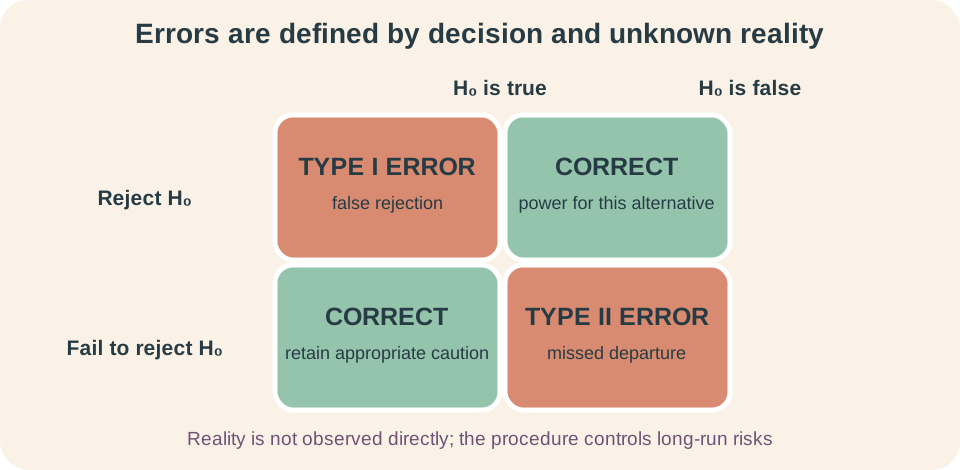
A Type I error occurs when a true null hypothesis is rejected. The selected significance level controls its probability under the null, subject to the assumptions and test procedure. In quality control, this might mean declaring a correctly centered process off target. The harm could include unnecessary shutdown or recalibration. The meaning of the error comes from the decision context.

A Type II error occurs when a false null is not rejected. Its probability is commonly written $\beta$, but unlike $\alpha$, it depends on which specific alternative value is true. In quality control, this could mean failing to detect a practically important shift. Larger departures are generally easier to detect than tiny ones. There is therefore no single Type II error probability without specifying an alternative scenario.

The two error types trade off when sample size and design remain fixed. Reducing $\alpha$ makes rejection harder and generally increases Type II error for a particular alternative. Increasing $\alpha$ does the reverse. Larger, better-measured samples can reduce both errors by increasing information. Error costs should influence design rather than being discussed only after results appear.

Understand power and study design

Power is the probability of rejecting the null when a specified alternative is true. It equals $1-\beta$ for that alternative, where $\beta$ is the corresponding Type II error probability. Power is a property of a procedure under an assumed effect, variability, sample size, significance level, and design. It is not a fixed label attached to a test name. A power statement must specify the effect it is intended to detect.

Power generally increases with larger true effects, larger sample sizes, lower measurement variability, and more efficient designs. It also usually increases with a larger significance level because rejection becomes easier. Paired or blocked designs can improve power by removing predictable variation. Better measurement can be as valuable as simply collecting more observations. Design choices determine how much information reaches the test statistic.

Prospective power analysis helps plan sample size before data collection. The target effect should be the smallest effect important enough to detect, not an unrealistically large effect chosen to justify a convenient sample. Post hoc power computed from the observed effect usually adds little beyond the p-value and confidence interval. After the study, uncertainty is better communicated through estimates and intervals. Power is primarily a design tool and a way to understand nondetection.

Separate statistical and practical significance

Statistical significance describes incompatibility with a null model at a chosen threshold. Practical significance asks whether the estimated effect matters in its real context. With a very large sample, a negligible effect may produce a tiny standard error and p-value. With a small sample, an important effect may remain uncertain. Neither p-value alone answers the practical question.

Report effect size in interpretable units. A mean difference of $0.10\,\mathrm{grams}$ may be irrelevant for one process and critical for another. Standardized effect sizes can support comparison across scales, but they do not replace original-unit interpretation. Costs, risks, biological relevance, and policy thresholds belong in the analysis. Statistical tools quantify uncertainty around a decision-relevant quantity.

Confidence intervals help unite magnitude and uncertainty. An interval may exclude zero yet contain only effects too small to matter. Another interval may include zero while also including large, consequential effects, indicating that the study is inconclusive rather than negative. Predefined practical margins make these distinctions clearer. Conclusions should state what effect sizes remain plausible.

Connect tests and confidence intervals

For many standard two-sided procedures, a level-$\alpha$ test rejects a candidate null value exactly when that value lies outside the corresponding $(1-\alpha)$ confidence interval. This duality requires matching estimators, standard errors, assumptions, and sidedness. A five-percent two-sided test commonly corresponds to a ninety-five-percent confidence interval. Both summarize the same sampling information from different directions. The test evaluates one candidate value, while the interval displays many compatible values.

If a ninety-five-percent confidence interval for a mean difference is $(0.4\,\mathrm{grams},2.0\,\mathrm{grams})$, then zero lies outside the interval. The matching two-sided null of zero difference would be rejected at the five-percent level. The interval also shows that supported effects range from modest to larger positive values. That magnitude information is absent from a bare rejection statement. Intervals therefore usually deserve prominence in reporting.

One-sided tests correspond to one-sided confidence bounds rather than automatically to the usual two-sided interval. Discrete tests and procedures with different approximations may not show exact numerical duality. Multiple-comparison adjustments also change the matching interval coverage. Do not combine a test and interval produced from incompatible methods. The logic matches only when the procedures match.

Account for multiple testing and selection

If twenty independent true null hypotheses are each tested at $\alpha=0.05$, the expected number of false rejections is one. The probability of at least one false positive is greater than five percent. Searching many outcomes, subgroups, time points, models, or stopping rules creates a similar selection problem. Reporting only the smallest p-value hides the effective number of opportunities. Transparency about the full analysis family is essential.

Familywise-error methods such as Bonferroni control the probability of at least one false rejection in a defined family. False-discovery-rate methods target the expected proportion of false discoveries among rejected hypotheses under their conditions. These goals are different, so the adjustment should match the scientific purpose. Planned primary outcomes usually deserve different status from exploratory analyses. Adjustment is not a substitute for a coherent study question.

Replication and validation address selection in another way. An exploratory pattern may generate a hypothesis that is evaluated in new data. Preregistration records primary questions and analysis choices before outcomes are known. Complete reporting allows readers to assess the search process. Evidence becomes stronger when the procedure that produced it is visible.

Diagnose common interpretation failures

The most serious mistake is interpreting $p$ as $P(H_0\mid\text{data})$. The p-value instead concerns $P(\text{data at least as extreme}\mid H_0)$ under a specified procedure. Conditional probabilities generally cannot be reversed without additional prior information and a probabilistic model for alternatives. Another mistake claims that $1-p$ is the probability of replication. Neither statement follows from the definition.

“Accept the null” is usually too strong after a nonsignificant test. The study may lack precision to distinguish a small effect from zero. Equivalence testing can support a claim that effects lie within a predefined negligible range, but ordinary failure to reject cannot. Examine the confidence interval and the study’s power for important alternatives. Ask what effects remain compatible with the evidence.

Other failures include choosing hypotheses after viewing data, ignoring dependence, reporting only significant outcomes, and equating significance with causation. Random assignment, not a small p-value, supplies the main design basis for a causal treatment claim. Random sampling, not significance, supports population generalization. Measurement validity remains necessary in every design. Inferential calculations cannot repair a poorly defined outcome or biased data source.

Practice complete hypothesis reasoning

Interpret $p=0.03$ for a two-sided test of a population mean. State which error occurs when a false null is not rejected. Explain why a trivially small effect can produce a tiny p-value in a very large sample. Distinguish $\alpha$ from the probability that a particular decision is wrong. Use complete sentences rather than only naming terms.

A random sample of $36$ packages has mean mass $100.8\,\mathrm{grams}$ and standard deviation $2.4\,\mathrm{grams}$. Test $H_0:\mu=100.0\,\mathrm{grams}$ against $H_A:\mu>100.0\,\mathrm{grams}$. Calculate the standard error and $t$ statistic with units shown before cancellation. Identify the reference distribution and degrees of freedom. State what additional information is needed before a contextual conclusion.

Suppose a ninety-five-percent confidence interval for a treatment difference is $(-0.2\,\mathrm{minutes},1.8\,\mathrm{minutes})$. Decide whether the matching two-sided five-percent test rejects zero. Explain why this is not proof that the treatment has no effect. If differences smaller than $0.5\,\mathrm{minutes}$ are practically negligible, identify which consequential values remain plausible. Describe one way to obtain more informative evidence.

Solutions and reasoning

If the null model and assumptions were true, a statistic at least as extreme in either specified tail would occur with probability $0.03$. Failing to reject a false null is a Type II error. Large samples reduce standard error, so even a tiny estimate-minus-null discrepancy can be many standard errors from zero. The significance level is the procedure’s long-run Type I error rate under the null. It is not the posterior error probability for one decision.

The standard error is $\frac{2.4\,\mathrm{grams}}{\sqrt{36}}=0.40\,\mathrm{grams}$. The statistic is $t=\frac{100.8\,\mathrm{grams}-100.0\,\mathrm{grams}}{0.40\,\mathrm{grams}}=2.00$. Under the null and conditions, use a $t$ distribution with $36-1=35$ degrees of freedom. Because the alternative is right-sided, the p-value uses the upper tail. A conclusion also requires checks of sampling, independence, distributional conditions, practical tolerances, and measurement quality.

Zero lies inside the interval, so the matching two-sided test does not reject at the five-percent level. The interval still allows effects from a small negative value through a positive value of $1.8\,\mathrm{minutes}$. Positive effects above the $0.5\,\mathrm{minute}$ practical threshold remain plausible. Therefore the result is inconclusive for practical benefit rather than proof of no effect. A larger or more precise well-designed study could narrow the interval.

Report evidence as a calibrated argument

A sound report identifies the parameter, population, hypotheses, design, estimator, and assumptions. It gives the test statistic, reference distribution, degrees of freedom when relevant, and p-value. It reports the effect estimate and confidence interval in original units. It distinguishes statistical evidence from practical importance. It limits causal and population claims to what the design supports.

Avoid reducing a conclusion to “significant” or “not significant.” State the direction and magnitude of the observed effect, its uncertainty, and how compatible the data are with the null model. Describe diagnostic limitations and any multiplicity or selection. Explain which consequences matter if a Type I or Type II error occurs. Readers need enough information to evaluate the argument independently. A calibrated conclusion makes those evidential and decision layers visible rather than hiding them behind a label.

Hypothesis testing is best understood as one component of evidence assessment. It calibrates a discrepancy under a reference model, but it does not assign truth, importance, or causation by itself. Confidence intervals, study design, measurement validity, prior evidence, and replication complete the picture. Keep those components visible at every step. The result will be more rigorous and more useful than a threshold alone.