Regression and Residuals

Regression is a disciplined way to describe how the typical value of one quantity changes with another. A fitted line summarizes the systematic pattern, while residuals preserve the variation that the line does not explain. The fitting calculation is therefore only the beginning of an analysis. A useful regression must also survive checks of its assumptions, uncertainty, scope, and practical meaning. This lesson develops that complete workflow rather than treating a line of best fit as an automatic conclusion.

Establish the regression questions

By the end of this lesson, you should be able to define a linear regression model and explain every symbol in it. You will calculate and interpret fitted values and residuals using their original response units. You will derive the least-squares slope and intercept from centered data. You will connect total, explained, and residual variation. You will also decide when a numerical summary is meaningful and when a diagnostic plot contradicts the model.

Regression begins with a focused question about two quantitative variables. The explanatory variable, written $x$, is used to describe or predict changes in the response variable, written $y$. This naming does not by itself establish that $x$ causes $y$. It only specifies the directional role of the variables in the model. Context and study design determine whether a causal interpretation is defensible.

A complete analysis asks more than whether the scatterplot slopes upward or downward. It asks whether the mean relationship is plausibly linear, whether variation remains reasonably stable, and whether observations can be treated as independent. It examines influential points and the range over which predictions are supported. It quantifies sampling uncertainty when the data arise from an appropriate random process. Finally, it reports limitations alongside conclusions.

Define the population model and its symbols

For paired observations $(x_i,y_i)$, a simple linear population model is $y_i=\beta_0+\beta_1x_i+\varepsilon_i$. The subscript $i$ identifies one observation among $n$ observed pairs. The parameter $\beta_0$ is the population intercept, and $\beta_1$ is the population slope. The error term $\varepsilon_i$ represents the observation’s departure from the population mean line. Greek letters emphasize that these population quantities are generally unknown.

The conditional mean statement is $E(Y\mid X=x)=\beta_0+\beta_1x$. The symbol $E$ means expected or long-run mean value, and the vertical bar means “given.” Thus the equation describes the mean response among cases having predictor value $x$. It does not claim that every observed response lies on the line. Individual variation is represented by the error term. That separation between a mean pattern and individual outcomes is fundamental to regression.

Units reveal what the parameters mean. If $y$ is fuel use in liters and $x$ is distance in kilometers, then $\beta_1$ has units $\frac{\mathrm{liters}}{\mathrm{kilometer}}$. Multiplying slope by distance produces liters, which can be added to the intercept measured in liters. The error term and response also carry liters. This dimensional agreement is necessary for the equation to represent the stated quantities.

Distinguish fitted values, errors, and residuals

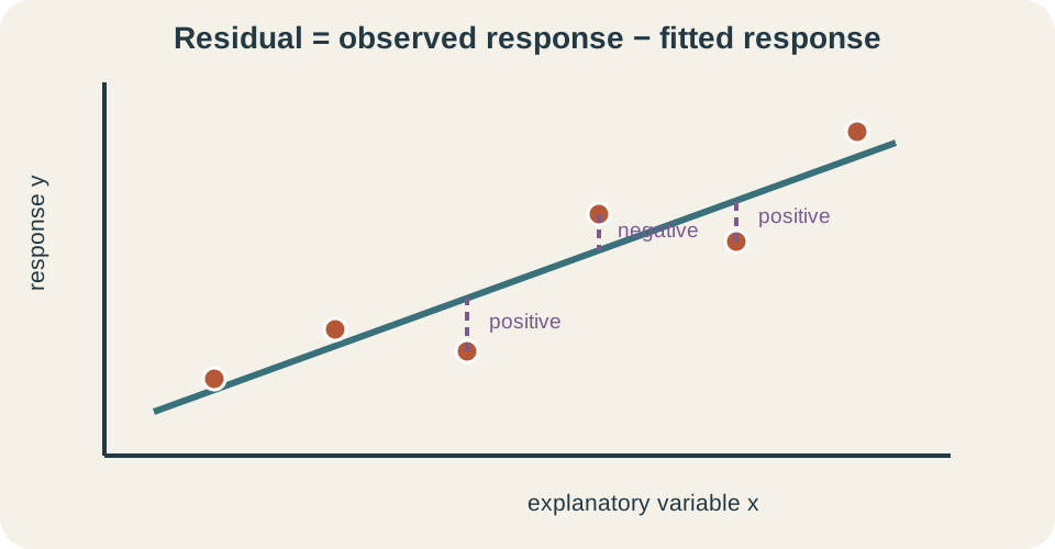
The fitted sample line is $\widehat y_i=b_0+b_1x_i$. The hat over $y$ indicates a predicted or fitted value rather than an observed response. The symbols $b_0$ and $b_1$ are estimates calculated from the sample. A residual is $e_i=y_i-\widehat y_i$, meaning observed response minus fitted response. This sign convention must remain consistent throughout the analysis.

A positive residual means the observed point lies above the fitted line because $y_i>\widehat y_i$. A negative residual means the point lies below the fitted line. A residual of zero means the fitted value exactly matches that observation. Residual magnitude is the vertical prediction discrepancy in response units. It is not the perpendicular geometric distance to the line.

Errors and residuals are related but not identical. The unobservable error $\varepsilon_i$ measures departure from the unknown population mean line. The observable residual $e_i$ measures departure from the fitted sample line. Because the same data determine the line and the residuals, residuals obey mathematical constraints not imposed on independent population errors. They are diagnostic proxies for the unobserved errors.

Understand the least-squares criterion

Least squares chooses $b_0$ and $b_1$ to minimize the residual sum of squares, $\operatorname{SSE}=\sum_{i=1}^{n}[y_i-(b_0+b_1x_i)]^2$. The capital sigma $\sum$ instructs us to add the following quantity over observations $i=1$ through $n$. The bracketed expression is the residual associated with a proposed line. Squaring makes every contribution nonnegative and penalizes larger discrepancies strongly. The acronym SSE means sum of squared errors, although the computed quantities are residuals.

Squaring also gives a smooth objective that can be differentiated. Without squaring, positive and negative residuals could cancel and falsely suggest a perfect fit. Absolute residuals provide another valid criterion, but they produce a different estimator with different mathematical properties. Least squares is common because its solution is explicit and its sampling theory is well developed. Its sensitivity to large residuals is both a feature and a vulnerability.

The fitting objective must match the measurement structure. Ordinary least squares measures vertical response discrepancies and treats the predictor values as fixed or measured without consequential error. If both coordinates contain important measurement error, a different modeling method may be required. If response variability changes substantially with $x$, weighted least squares may be more suitable. Selecting a criterion is a modeling decision, not merely a software default.

Derive the slope from centered variation

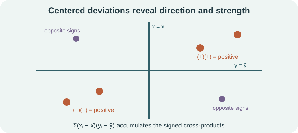
Minimizing SSE produces $b_1=\frac{\sum_{i=1}^{n}(x_i-\overline x)(y_i-\overline y)}{\sum_{i=1}^{n}(x_i-\overline x)^2}$. The bars in $\overline x$ and $\overline y$ denote sample means. Each centered value $x_i-\overline x$ records a predictor deviation from its mean, while $y_i-\overline y$ records a response deviation. The numerator accumulates whether those deviations tend to share signs. The denominator measures the predictor’s total squared spread.

If large $x$ values tend to accompany large $y$ values and small $x$ values accompany small $y$ values, the cross-products are mostly positive. The fitted slope is then positive. Opposite-signed deviations produce a negative numerator and negative slope. A predictor with no variation makes the denominator zero, so no slope can be estimated. Regression requires variation in the explanatory variable.

The intercept is $b_0=\overline y-b_1\overline x$. Substituting $x=\overline x$ into the fitted equation gives $\widehat y=\overline y$, so the least-squares line passes through $(\overline x,\overline y)$. This fact is a useful check on a calculation. It also explains why centering $x$ can make an intercept more interpretable. The formulas arise from minimizing the objective, not from visually balancing the points.

Interpret slope and intercept with units

Suppose predicted fuel use is $\widehat F=2.1\,\mathrm{liters}+(0.075\,\frac{\mathrm{liters}}{\mathrm{kilometer}})d$, where $d$ is distance. Within the observed range, predicted fuel use increases by $0.075\,\mathrm{liters}$ for each additional kilometer. The phrase “predicted” matters because individual journeys vary around the fitted relationship. The unit ratio describes change in response per unit change in predictor. A slope statement should name both quantities and the relevant population or context.

The intercept predicts $2.1\,\mathrm{liters}$ when $d=0\,\mathrm{kilometers}$. Whether that value is scientifically meaningful depends on how fuel use and journeys were defined. It might represent idling, startup consumption, or an extrapolation artifact. An intercept remains algebraically necessary even when zero lies outside the observed predictor range. Interpretation should never outrun the data context.

For $d=100\,\mathrm{kilometers}$, substitution gives $\widehat F=2.1\,\mathrm{liters}+(0.075\,\frac{\mathrm{liters}}{\mathrm{kilometer}})(100\,\mathrm{kilometers})=9.6\,\mathrm{liters}$. Kilometer units cancel inside the product, leaving liters. If the observed use is $10.4\,\mathrm{liters}$, the residual is $10.4\,\mathrm{liters}-9.6\,\mathrm{liters}=0.8\,\mathrm{liters}$. The positive sign states that the model underpredicted this journey. Units make every numerical quantity interpretable.

Decompose response variation

With an intercept in the model, total variation is $\operatorname{SST}=\sum_{i=1}^{n}(y_i-\overline y)^2$. The acronym SST means total sum of squares. Explained variation is $\operatorname{SSR}=\sum_{i=1}^{n}(\widehat y_i-\overline y)^2$. Residual variation is $\operatorname{SSE}=\sum_{i=1}^{n}(y_i-\widehat y_i)^2$. All three quantities have squared response units.

Ordinary least squares with an intercept satisfies $\operatorname{SST}=\operatorname{SSR}+\operatorname{SSE}$. Geometrically, the fitted and residual components are orthogonal in observation space. Informally, total deviations around the response mean separate into modeled deviations and leftover deviations. This exact decomposition depends on the fitting setup. It should not be assumed automatically for every model or every definition of fit.

The coefficient of determination is $R^2=\frac{\operatorname{SSR}}{\operatorname{SST}}=1-\frac{\operatorname{SSE}}{\operatorname{SST}}$. It describes the proportion of in-sample response variation accounted for by the fitted linear model. If $\operatorname{SST}=200\,\mathrm{liters}^2$ and $\operatorname{SSE}=50\,\mathrm{liters}^2$, then $R^2=1-\frac{50}{200}=0.75$. The fraction is dimensionless because squared response units cancel. The result does not prove causality, good calibration, or future predictive accuracy.

Measure residual scale responsibly

The residual standard error is $s=\sqrt{\frac{\operatorname{SSE}}{n-2}}$ for simple linear regression with an intercept and slope. The denominator $n-2$ is the residual degrees of freedom because two coefficients were estimated. Taking the square root returns the measure to the original response unit. Thus an $s$ of $1.4\,\mathrm{liters}$ describes a typical residual scale in liters. It should be interpreted relative to the application’s meaningful error tolerance.

Root mean squared error is closely related but may use a different denominator depending on context. Training RMSE often divides by $n$, while inferential residual standard error divides by residual degrees of freedom. A reported number should therefore name its definition. Comparing values across datasets with different response units or scales can be misleading. Standardization or a context-specific benchmark may be needed.

No single fit statistic can validate a model. A small residual scale may coexist with systematic curvature if the response range is narrow. A high $R^2$ may coexist with biased predictions, influential observations, or extrapolation. Conversely, a modest $R^2$ can occur in a useful model for a naturally variable process. Numerical summaries must be read alongside plots and subject knowledge.

Read residual plots as model checks

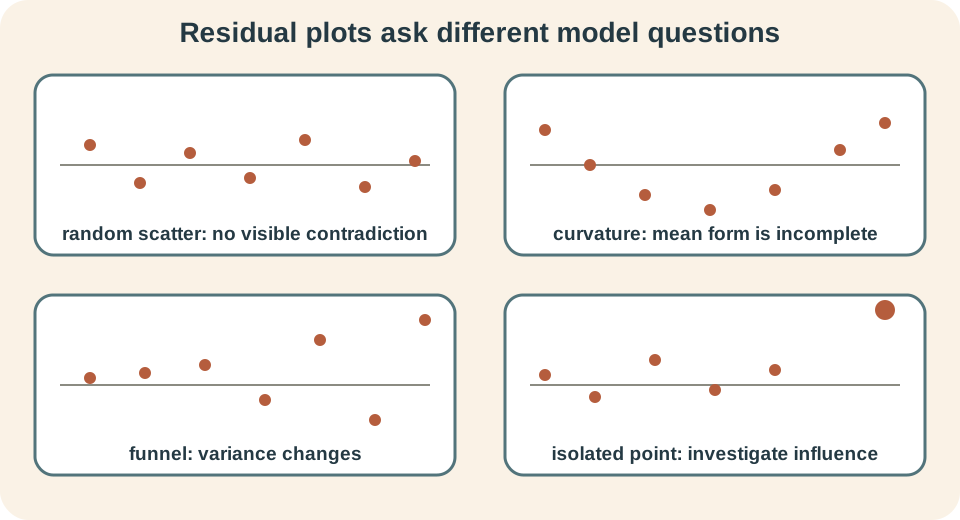
A residual plot places predictor values or fitted values on the horizontal axis and residuals on the vertical axis. A credible linear mean model should leave residuals fluctuating without systematic curvature around zero. A curved pattern indicates that the model misses structure in the mean relationship. Adding an arbitrary polynomial is not automatically the answer. The revised form should be supported by context and verified on new data when prediction matters.

A funnel shape indicates that residual spread changes with the fitted level or predictor. This pattern is called heteroscedasticity, meaning nonconstant conditional variance. Standard errors and intervals derived under constant variance may then be inaccurate. A transformation, variance model, robust standard error, or weighted fit may be appropriate. The choice depends on the data-generating process.

Time-ordered waves or runs suggest dependence among errors. Separate clusters may reveal an omitted group variable. An isolated point with unusual predictor value may exert high leverage, while a point that substantially changes estimates is influential. These concepts overlap but are not synonyms. Diagnostics should identify what feature is unusual and how conclusions change when it is investigated.

Connect assumptions to inference

Slope tests and confidence intervals commonly rely on a linear conditional mean, independent observations or appropriately modeled dependence, and valid standard-error estimation. Classical small-sample procedures additionally assume normally distributed errors with constant variance. Normality concerns the conditional errors, not necessarily the raw response distribution. Large samples can reduce sensitivity to some deviations but do not repair dependence or systematic misspecification. Assumptions must be connected to the procedure being used.

The estimated standard error of $b_1$ measures sampling variability in the fitted slope under the model. A test statistic compares the estimated slope with a hypothesized value in standard-error units. A confidence interval gives a range of slope values compatible with the sample and assumptions. Statistical significance does not measure practical importance. Units and domain context remain essential when interpreting the interval.

Observational association is not automatically causal. Confounding variables can influence both predictor and response, reverse causation can operate, and selection mechanisms can distort the observed pattern. Random assignment supports causal comparison because it balances confounders probabilistically. Random sampling supports population generalization when implementation is sound. Regression cannot manufacture design strength that the study does not possess.

Distinguish confidence and prediction intervals

A confidence interval at predictor value $x_0$ estimates the mean response $E(Y\mid X=x_0)$. It accounts for uncertainty in the estimated mean line. A prediction interval estimates one new individual response at $x_0$. It must include both uncertainty in the mean estimate and individual outcome variability. Therefore the prediction interval is wider under the same confidence level and model.

Both intervals are typically narrowest near $\overline x$ because the data provide the strongest leverage for estimating the mean there. They widen as $x_0$ moves away from the predictor mean. Far outside the observed range, formula-based intervals may look precise while relying on an untested linear form. The calculation does not protect against structural extrapolation error. The observed predictor range should accompany reported predictions.

Prediction quality should be assessed on data not used to fit the model when possible. Training residuals are optimistically small because the fitted coefficients were chosen to reduce them. A validation set or cross-validation estimates performance on new cases more honestly. The validation process must preserve dependence structures such as time, groups, or repeated measurements. Random splitting is not appropriate for every design.

Work through a small regression example

Consider distances $x=(1,2,3)$ kilometers and fuel amounts $y=(1.0,1.5,2.0)$ liters. Their means are $\overline x=2\,\mathrm{kilometers}$ and $\overline y=1.5\,\mathrm{liters}$. Centered predictor values are $(-1,0,1)$ kilometers, and centered responses are $(-0.5,0,0.5)$ liters. The numerator of the slope is $1.0\,\mathrm{liter}\!\cdot\!\mathrm{kilometer}$. The denominator is $2\,\mathrm{kilometers}^2$.

The slope is therefore $b_1=0.5\,\frac{\mathrm{liters}}{\mathrm{kilometer}}$. The intercept is $b_0=1.5\,\mathrm{liters}-(0.5\,\frac{\mathrm{liters}}{\mathrm{kilometer}})(2\,\mathrm{kilometers})=0.5\,\mathrm{liters}$. The fitted line is $\widehat y=0.5\,\mathrm{liters}+(0.5\,\frac{\mathrm{liters}}{\mathrm{kilometer}})x$. Each observed point lies exactly on this line. Consequently, all three residuals and SSE equal zero.

This perfect fit does not establish a universal physical law. Three points were deliberately chosen to be collinear, and no repeated measurements reveal natural variation. Predictions beyond three kilometers assume the same linear relationship continues. Real fuel data would usually include measurement uncertainty and operating differences. The example demonstrates calculation, while model credibility still requires broader evidence.

Diagnose common regression mistakes

Defining residual as fitted minus observed reverses every diagnostic sign. Always write $e=y-\widehat y$ before calculating. Another mistake interprets $R^2$ as the percentage of individual outcomes predicted correctly. It instead concerns variation around the sample response mean under the fitted model. A third mistake reports a unitless slope even when both variables are measured quantities.

Analysts may also ignore influential observations because the overall fit statistic remains large. Remove no point merely because it is inconvenient. Verify the observation, investigate its context, and report how conclusions depend on it. Robustness analysis is more informative than silent deletion. Unusual observations may expose either data problems or important scientific mechanisms.

Extrapolation and causal overstatement are especially serious. A regression estimated among observed adults may not describe children, other populations, or future conditions. A strong association can result from a lurking variable. Software output cannot determine the target population or causal design. Those conclusions require reasoning beyond the fitted coefficients.

Practice fitting and interpretation

If an observed response is $10\,\mathrm{grams}$ and its fitted value is $12\,\mathrm{grams}$, calculate and interpret the residual. If $\operatorname{SST}=200\,\mathrm{grams}^2$ and $\operatorname{SSE}=50\,\mathrm{grams}^2$, calculate $R^2$ and explain its scope. State what a curved residual plot suggests. Distinguish that pattern from a funnel-shaped plot. Give every numerical result its proper unit or explain why it is dimensionless.

Suppose $\widehat T=18\,\mathrm{degrees\ Celsius}+(0.6\,\frac{\mathrm{degrees\ Celsius}}{\mathrm{hour}})h$ models temperature after $h$ hours. Interpret the slope and intercept. Predict temperature at $h=5.0\,\mathrm{hours}$ and calculate the residual if the observed temperature is $20\,\mathrm{degrees\ Celsius}$. Decide whether a prediction at $h=100\,\mathrm{hours}$ is justified from data collected only between zero and eight hours. Explain the role of the observed range.

Finally, write a short regression report outline. It should identify the variables, population, units, design, fitted relationship, uncertainty, residual evidence, and limitations. Include a statement about causation appropriate for an observational study. Include a statement about where prediction is supported. This exercise emphasizes that regression is an argument assembled from several forms of evidence.

Solutions and reasoning

The residual is $e=10\,\mathrm{grams}-12\,\mathrm{grams}=-2\,\mathrm{grams}$, so the model overpredicted by two grams. The coefficient is $R^2=1-\frac{50}{200}=0.75$, and squared-gram units cancel. Thus the fitted model accounts for seventy-five percent of the in-sample response variation around its mean. Curvature suggests a missing nonlinear mean pattern. Funneling instead suggests changing residual variance.

The slope predicts an increase of $0.6\,\mathrm{degrees\ Celsius}$ per additional hour within the supported range. The intercept predicts $18\,\mathrm{degrees\ Celsius}$ at zero hours. At five hours, $\widehat T=18\,\mathrm{degrees\ Celsius}+(0.6\,\frac{\mathrm{degrees\ Celsius}}{\mathrm{hour}})(5.0\,\mathrm{hours})=21\,\mathrm{degrees\ Celsius}$. The residual is $20\,\mathrm{degrees\ Celsius}-21\,\mathrm{degrees\ Celsius}=-1\,\mathrm{degree\ Celsius}$. Prediction at one hundred hours is unsupported extrapolation because the linear form has not been observed there.

A sound report defines the explanatory and response variables with units and identifies how observations entered the sample. It gives the fitted equation and interprets coefficients in context. It summarizes residual scale and the diagnostic plots rather than reporting only $R^2$. It provides intervals or validation results suited to the inferential or predictive goal. For observational data, it describes association without claiming causation and limits prediction to a defensible population and range.

Carry the workflow forward

Regression proceeds through a sequence: define the question, inspect the data, specify the model, estimate its parameters, and interrogate the residuals. Each step can reveal a reason to revise the previous one. The fitted line is not a verdict but a proposed description. Diagnostics ask what the description leaves behind. Uncertainty and validation ask how stable it will be beyond the observed sample.

Later lessons extend this framework rather than replacing it. Nonlinear least squares changes the form of the mean function. Gauss–Newton and Levenberg–Marquardt provide iterative methods when coefficients no longer have a simple closed-form solution. ANOVA organizes variation and degrees of freedom, while information criteria compare fit against complexity. The habits learned here remain central in every extension.

Keep residuals at the center of your reasoning. Translate their signs, patterns, and scales back into the original context. Explain every statistic’s numerator, denominator, unit, and limitation. Separate descriptive association, statistical inference, prediction, and causal explanation. A regression becomes trustworthy only when the reasoning around the fitted equation is as careful as the calculation that produced it.