Random Variables and Distributions

A random variable turns outcomes of an uncertain process into numbers that can be analyzed. The mapping is fixed even though the outcome is not known in advance. A probability distribution then describes how probability is allocated among possible numerical values or intervals. Expected value summarizes center, while variance and standard deviation summarize spread. This lesson connects outcome spaces, functions, graphs, calculations, assumptions, and interpretation.

Begin with outcomes and a fixed mapping

An experiment is any repeatable or conceptually repeatable process with an uncertain outcome. Its sample space $\Omega$ is the set of possible outcomes. The Greek capital omega, $\Omega$, is a conventional symbol for that space. An event is a subset of outcomes. Probability is assigned to events before a random variable converts outcomes into numerical values.

A random variable is a function $X:\Omega\to\mathbb R$. The arrow means that $X$ maps each outcome in the sample space to one real number. The capital letter $X$ names the random variable. A lowercase $x$ commonly represents one possible numerical value. Randomness lies in which outcome occurs, not in whether the mapping changes its rule.

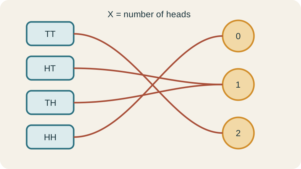
For two coin tosses, the sample space is $\{HH,HT,TH,TT\}$. Define $X$ as the number of heads. Then $X(HH)=2$, $X(HT)=1$, $X(TH)=1$, and $X(TT)=0$. Different outcomes can map to the same numerical value. The distribution combines their probabilities after the mapping.

Distinguish random variables from their realized values

Before an outcome is observed, $X$ represents a numerical quantity whose value is uncertain. After observation, a realized value such as $x=1$ can be recorded. The statement $X=1$ describes the event containing every outcome mapped to one. For the two-toss example, that event is $\{HT,TH\}$. Probability can therefore be written $P(X=1)$.

The random variable is not itself a probability. It is a numerical function to which probabilities are transferred from outcomes. A value such as $X=2$ can have a probability, but the number two is not a probability. Keeping function, value, event, and probability separate prevents notation from collapsing. Each object plays a different role.

Random variables can carry physical units. If $X$ is waiting time, it may be measured in seconds. If $Y$ is mass, it may be measured in kilograms. Probabilities are dimensionless, while density units depend on the variable. Expected values inherit the variable’s units.

Classify discrete and continuous variables

A discrete random variable has a finite or countably infinite set of possible values. Counts such as number of defects, number of arrivals, or number of successes are usually discrete. The values may be listed in principle even if the list is infinite. Gaps can exist between possible values. Probability may be assigned directly to individual values.

A continuous random variable can take values across intervals. Idealized measurement quantities such as time, length, temperature, or concentration are often modeled continuously. Any one exact value has probability zero under a continuous density model. Intervals can still have positive probability. Probability comes from area rather than from density height alone.

The distinction belongs to the model as well as the measurement. A digital instrument may record temperature to the nearest $0.1\,^{\circ}\mathrm{C}$, producing discrete recorded values. A continuous model may remain a useful approximation to the underlying temperature. Modeling choices simplify reality for a purpose. Their consequences should be acknowledged.

Construct a probability mass function

For a discrete random variable $X$, the probability mass function is $p_X(x)=P(X=x)$. The subscript reminds the reader which random variable the function describes. Every mass satisfies $p_X(x)\geq0$. The masses sum to one, written $\sum_xp_X(x)=1$. The sigma symbol instructs us to add over every possible value.

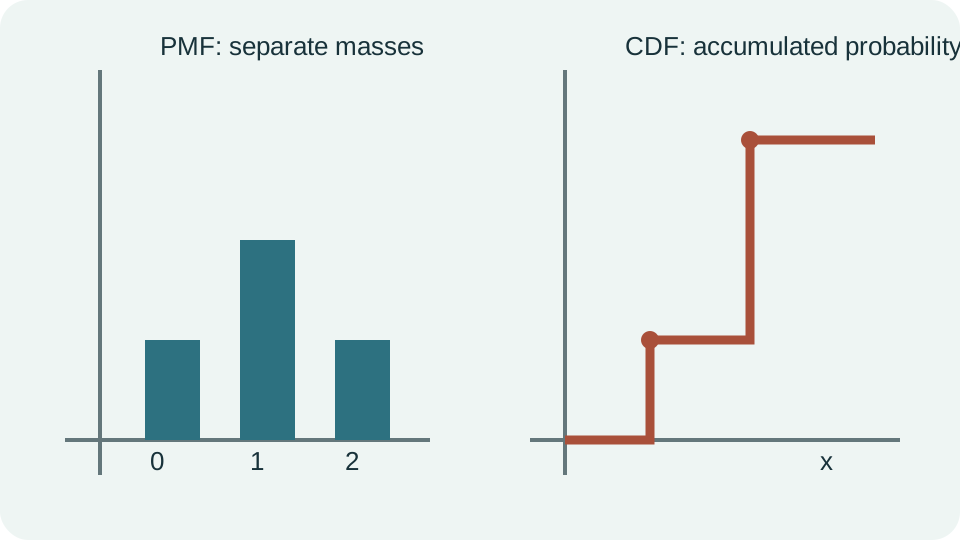
For the number of heads in two fair tosses, $p_X(0)=\dfrac{1}{4}$, $p_X(1)=\dfrac{1}{2}$, and $p_X(2)=\dfrac{1}{4}$. The middle value receives probability from two outcomes. Adding gives $\dfrac{1}{4}+\dfrac{1}{2}+\dfrac{1}{4}=1$. No probability belongs to values outside zero, one, and two. A bar graph can display the separate masses.

The mass function provides probabilities of events by addition. For example, $P(X\geq1)=p_X(1)+p_X(2)=\dfrac{3}{4}$. The symbol $\geq$ means greater than or equal to. The event includes one or two heads. Discreteness makes endpoint inclusion visible because individual points can carry probability.

Use the cumulative distribution function

The cumulative distribution function is $F_X(x)=P(X\leq x)$. It records all probability at or below the input value. The definition works for discrete, continuous, and mixed variables. A CDF never decreases as $x$ increases. Its values lie between zero and one.

For a discrete variable, the CDF is a step function. It jumps at each value with positive probability. The jump size at $x$ equals $P(X=x)$. Between possible values, the CDF stays constant. Right-continuity determines how each jump endpoint is included.

Interval probabilities can be recovered through subtraction. For $a<b$, $P(a<X\leq b)=F_X(b)-F_X(a)$. The left endpoint is excluded because $F_X(a)$ removes probability at or below $a$. Different endpoint choices matter for discrete variables. For a continuous distribution, individual endpoints have zero probability and the choices agree.

Define a continuous probability density

A continuous random variable can be described by a probability density function $f_X(x)$. The density must satisfy $f_X(x)\geq0$. Its total area is one, written $\int_{-\infty}^{\infty}f_X(x)\,dx=1$. The integral sign represents continuous accumulation. Infinite limits mean the entire real line is included.

Probability over an interval is $P(a\leq X\leq b)=\int_a^bf_X(x)\,dx$. The probability is area under the density curve between the endpoints. Density height is probability per unit of $x$, not probability at one point. A density can exceed one if it remains narrow enough that total area is one. Only accumulated area must lie between zero and one.

If $X$ is measured in seconds, density has units of inverse seconds. Multiplying density by the differential width $dx$ produces a dimensionless probability contribution. This unit analysis explains why density height is not itself probability. Changing measurement units changes numerical density height. The same interval probability remains invariant after proper transformation.

Understand zero probability at a point

For a continuous variable, $P(X=x)=0$ for every exact value $x$. This does not mean that the variable can never take a value. It means an individual point has zero width and therefore zero density area. Uncountably many zero-probability points collectively form intervals with positive probability. The logic differs from adding a countable list of zeros.

Measurement language often rounds continuous values. An instrument reading $5.0\,\mathrm{s}$ may represent an interval such as $4.95\,\mathrm{s}\leq X<5.05\,\mathrm{s}$. That interval can have positive probability. The displayed number is not an infinitely precise event. Resolution links continuous models with discrete records.

For continuous $X$, endpoint inclusion does not affect interval probability. Thus $P(a<X<b)=P(a\leq X\leq b)$ under the model. For discrete $X$, adding or removing an endpoint may change probability. Recognizing the variable type determines whether inequality symbols matter numerically. This is a conceptual check before integration or summation.

Calculate expected value for discrete variables

The expected value of a discrete random variable is $E[X]=\sum_xx\,p_X(x)$ when the sum exists. Each possible value is multiplied by its probability and the products are added. The operator $E$ means expectation. Expected value is a probability-weighted center. It is not necessarily one of the possible outcomes.

For the two-toss head count, $E[X]=0\left(\dfrac{1}{4}\right)+1\left(\dfrac{1}{2}\right)+2\left(\dfrac{1}{4}\right)=1$. In this case, the expectation is a possible value. For a fair six-sided die, expectation is $3.5$ even though no face displays $3.5$. The value describes long-run average behavior across repeated independent trials. It does not predict the next outcome.

Expectation is linear. For constants $a$ and $b$, $E[aX+b]=aE[X]+b$. This rule does not require independence because only one variable appears. More generally, $E[X+Y]=E[X]+E[Y]$ even when $X$ and $Y$ are dependent. Linearity makes totals easier to analyze than their full distributions.

Calculate expectation for continuous variables

For a continuous random variable, expectation is $E[X]=\int_{-\infty}^{\infty}x f_X(x)\,dx$ when the integral exists. The value $x$ is weighted by density and accumulated over the real line. The formula parallels the discrete probability-weighted sum. Integrals replace sums because values vary continuously. The result inherits the units of $X$.

Suppose $X$ is uniform on $[0,4\,\mathrm{s}]$. Its density is $f_X(x)=\dfrac{1}{4\,\mathrm{s}}$ over that interval and zero elsewhere. The expectation is $\int_0^{4\,\mathrm{s}}x\left(\dfrac{1}{4\,\mathrm{s}}\right)dx=2\,\mathrm{s}$. Symmetry also places the center halfway between the endpoints. Units reduce correctly during integration.

An expectation need not exist even when a valid probability distribution exists. Heavy tails can make the positive and negative weighted contributions fail to converge. A distribution also can have a mean but no finite variance. Formulas require existence conditions. Software output should not replace checking those mathematical assumptions.

Interpret expected value in decisions

Consider a game that pays $8.00\,\mathrm{dollars}$ with probability $0.25$ and loses $3.00\,\mathrm{dollars}$ with probability $0.75$. Let net payoff be $X$. Its expected value is $E[X]=(8.00\,\mathrm{dollars})(0.25)+(-3.00\,\mathrm{dollars})(0.75)=-0.25\,\mathrm{dollars}$. Over many independent plays, average payoff tends toward a loss of about twenty-five cents per play. One play still produces either gain or loss.

Expected monetary value is not the only decision criterion. A rare catastrophic loss can matter more than its average contribution suggests. Risk tolerance, utility, legal constraints, and resource limits may alter a rational choice. Two distributions with the same expectation can have very different spreads and tails. Center must be interpreted with variability.

Expectation can also describe conservation across random outcomes. If repeated fair transfers redistribute money without external cost, total expected money may remain fixed. Individual outcomes can still vary substantially. Expected value summarizes an ensemble or long-run average. It does not make uncertainty disappear.

Define variance and standard deviation

Let $\mu=E[X]$ denote the population mean. Variance is $\operatorname{Var}(X)=E[(X-\mu)^2]$. The difference $X-\mu$ measures deviation from the mean. Squaring prevents positive and negative deviations from canceling. Averaging squared deviations quantifies spread.

Variance has squared units. If $X$ is measured in meters, variance is measured in square meters. Standard deviation is $\sigma=\sqrt{\operatorname{Var}(X)}$. The Greek letter sigma, $\sigma$, commonly denotes population standard deviation. Taking the square root returns to the original units.

The computational identity is $\operatorname{Var}(X)=E[X^2]-\mu^2$ when the required expectations exist. It follows by expanding $(X-\mu)^2$ and using linearity of expectation. The identity can simplify hand calculations. In floating-point computation with very large nearly equal terms, a numerically stable algorithm may be preferable. Algebraic equivalence does not guarantee identical numerical behavior under finite precision.

Compute a discrete variance

Let $P(X=0)=0.2$, $P(X=1)=0.5$, and $P(X=2)=0.3$. The mean is $\mu=0(0.2)+1(0.5)+2(0.3)=1.1$. Next compute $E[X^2]=0^2(0.2)+1^2(0.5)+2^2(0.3)=1.7$. Therefore variance is $1.7-(1.1)^2=0.49$. The standard deviation is $0.70$.

If $X$ counts events, the mean and standard deviation are expressed in count units, while variance is in squared count units. The calculation uses population probabilities rather than a sample denominator correction. Every probability contributes to both moments. A probability table helps prevent omitted values. The probabilities should sum to one before moments are trusted.

The mean $1.1$ is not required to be an attainable count. It locates the distribution’s balance point. The standard deviation $0.70$ describes a typical scale of variation but is not a strict boundary. Individual values can lie more than one standard deviation away. Distribution shape determines how probability is arranged around the center.

Transform location and scale

Let $Y=aX+b$, where $a$ and $b$ are constants. The expectation is $E[Y]=aE[X]+b$. Adding $b$ shifts every value and therefore shifts the mean by $b$. Multiplying by $a$ scales all values and the mean. Units must remain compatible when quantities are added.

Variance transforms as $\operatorname{Var}(Y)=a^2\operatorname{Var}(X)$. The shift $b$ does not affect spread because it moves every value equally. The factor $a$ is squared because deviations are squared. Standard deviation becomes $\sigma_Y=|a|\sigma_X$. Absolute value keeps spread nonnegative when $a$ is negative.

If $E[X]=4.0\,\mathrm{m}$ and $\operatorname{Var}(X)=9.0\,\mathrm{m^2}$, let $Y=2X-1.0\,\mathrm{m}$. Then $E[Y]=7.0\,\mathrm{m}$. The variance is $4(9.0\,\mathrm{m^2})=36\,\mathrm{m^2}$. The standard deviation changes from $3.0\,\mathrm{m}$ to $6.0\,\mathrm{m}$. Subtracting $1.0\,\mathrm{m}$ shifts the center but contributes nothing to the spread.

Recognize common discrete models

A Bernoulli random variable records one success or failure. It takes value one with probability $p$ and zero with probability $1-p$. Its mean is $p$, and its variance is $p(1-p)$. The word success labels the event of interest without implying desirability. The model represents one binary trial.

A binomial variable counts successes in $n$ independent Bernoulli trials with constant success probability $p$. Its mean is $np$, and its variance is $np(1-p)$. Independence and constant probability are substantive assumptions. Sampling without replacement from a small population generally violates independence. Changing trial conditions can invalidate constant $p$.

A geometric variable models the number of trials until the first success under repeated independent equal-probability trials. A Poisson variable often models counts of events in a fixed exposure when a constant-rate and independence structure is plausible. Each distribution is a model with assumptions, not merely a formula shape. Context should be checked before parameters are estimated. Similar-looking count data can arise from different processes.

Recognize common continuous models

The uniform distribution assigns constant density across a finite interval. Equal-length subintervals then have equal probability. The normal distribution has a symmetric bell shape determined by mean $\mu$ and standard deviation $\sigma$. It extends over the entire real line. Many measurement and aggregation processes are approximately normal in central regions.

An exponential distribution models nonnegative waiting times under a constant-rate memoryless process. Its density decreases as time increases. A lognormal distribution models positive quantities whose logarithms are approximately normal. It often has a long right tail. Choosing among these models requires process knowledge and diagnostic checking.

Normality should not be assumed merely because a histogram looks vaguely bell shaped. Sample size, bin choices, tails, truncation, and mixtures can mislead. Quantile plots and subject knowledge provide additional evidence. Even an approximate model may be useful for one purpose and poor for another. The relevant features depend on the intended calculation.

Connect distributions to graphs and simulation

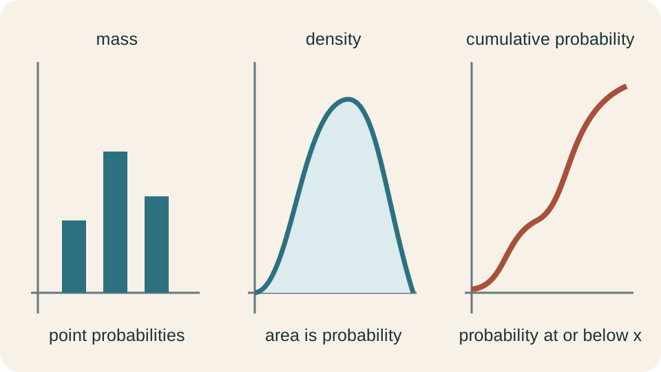
A PMF graph uses separated bars or points because discrete values carry masses. A density graph uses a continuous curve whose areas represent probability. A CDF graph always rises from near zero toward one. These graphs encode different objects. Their vertical axes should not be labeled interchangeably.

Simulation generates outcomes according to a specified distribution. Repeated simulated values form empirical frequencies and averages. As the number of trials grows, these summaries often approach theoretical probabilities and expectations under appropriate conditions. Simulation can build intuition and approximate difficult calculations. It does not validate whether the chosen distribution describes reality.

Empirical distributions summarize observed or simulated data without asserting a smooth theoretical family. The empirical CDF increases by observation weights at recorded values. Comparing it with a fitted model can reveal discrepancies. Graphical comparison is strongest when paired with context and uncertainty. A model is a proposed data-generating description, not the data themselves.

Diagnose common probability mistakes

One mistake is treating density height as probability. Only an integral over an interval gives continuous probability. Another is expecting the mean to be a possible outcome. The mean is a weighted center and can lie between attainable values. A third is forgetting that standard deviation, not variance, shares the variable’s units.

Another mistake is failing to square a scale factor in variance. If values double, deviations double and squared deviations quadruple. A shift changes the mean but not spread. Unit analysis makes these transformations easier to remember. Variance units expose a missing square.

Model assumptions also cause errors. A binomial model requires a fixed number of trials, binary outcomes, independence, and constant success probability. A normal model can assign impossible negative values to inherently positive quantities if variability is large. A distribution name should be accompanied by an argument for why its structure applies. Calculation cannot repair a mismatched model.

Practice a complete distribution routine

First define the experiment, sample space, and random-variable mapping. Second classify the numerical variable as discrete or continuous under the chosen model. Third specify a PMF, density, or CDF with domain and units. Fourth check nonnegativity and total probability one. Fifth calculate the requested probability or moment and interpret it in context.

Suppose delivery time $T$ is uniform from $4.0\,\mathrm{min}$ to $10.0\,\mathrm{min}$. The density is $\dfrac{1}{6.0\,\mathrm{min}}$ over that interval. The probability of delivery between $5.0\,\mathrm{min}$ and $8.0\,\mathrm{min}$ is interval width divided by total width, or $\dfrac{3.0\,\mathrm{min}}{6.0\,\mathrm{min}}=0.50$. The mean is the midpoint $7.0\,\mathrm{min}$. Units cancel in probability but remain in expectation.

As a discrete check, let $X$ count successes in ten independent trials with $p=0.30$. A binomial model gives $E[X]=np=3.0$. Its variance is $np(1-p)=2.1$, and standard deviation is $\sqrt{2.1}=1.45$. These summaries do not imply that every outcome lies between roughly one and four successes. The complete distribution is needed for exact event probabilities.

Consolidate distribution reasoning

A random variable maps outcomes to numbers. A PMF assigns probability mass to discrete values, while a density assigns probability per unit to continuous regions. A CDF accumulates probability at or below each input and works for either type. Expected value locates a weighted center. Variance and standard deviation quantify spread on squared and original scales.

Transformations change center and spread in predictable ways. Common distribution families package particular assumptions about support, independence, rate, symmetry, and tail behavior. Their formulas become meaningful only when those assumptions fit the process. Graphs and simulation help compare representations. Units keep probabilities, densities, values, and moments distinct.

The strongest solution begins with the outcome process and mapping rather than with a memorized distribution name. It checks normalization, support, endpoint meaning, and dimensional consistency. It interprets averages as long-run or ensemble centers rather than guarantees for individuals. Probability distributions organize uncertainty without eliminating it. Their value lies in making assumptions and consequences explicit.