Conditional Probability

Probability is not merely a list of fixed numbers attached to events. A probability describes uncertainty relative to the information currently available. When new information rules out some outcomes, the relevant sample space changes, so the probabilities within it must be recalculated. Conditional probability is the mathematical language for performing that update without losing track of the original experiment. The central habit of this lesson is therefore simple: identify the new universe of possible outcomes before doing arithmetic.

Learning objectives and a guiding question

By the end of this lesson, you will be able to interpret and calculate a conditional probability from words, tables, trees, and formulas. You will derive and use the multiplication rule, distinguish independence from disjointness, and combine cases with the law of total probability. You will also use Bayes’ theorem to reverse the direction of a condition while respecting prior probabilities. Every formula will be connected to a restricted sample space so that the notation records reasoning rather than replacing it. These skills prepare you for probability distributions, statistical inference, reliability analysis, and evidence-based decision making.

The guiding question is, “What remains possible after I learn this information?” Suppose a card is selected from a standard deck and you are told that the card is a face card. The original sample space contained $52$ equally likely cards, but only $12$ face cards remain compatible with the information. If the question asks for the probability that the card is a king, the relevant count is four kings out of those twelve remaining cards. The answer is therefore the horizontal fraction $\frac{4}{12}=\frac{1}{3}$, not $\frac{4}{52}$. The new information has changed the denominator from fifty-two to twelve.

This example contains the entire conceptual structure of conditioning. The phrase “given that the card is a face card” identifies the restricted universe. The desired event, drawing a king, is then intersected with that universe because an outcome must satisfy both descriptions. The denominator measures the size or probability of the given event, while the numerator measures the part that also satisfies the target event. Before memorizing any rule, practice saying those two roles aloud.

From a sample space to a restricted sample space

Let $S$ denote the original sample space, and let $A$ and $B$ be events within it. Learning that $B$ occurred removes every outcome outside $B$ from consideration. The event $B$ therefore acts as the new sample space, even though the original probability model was built on $S$. The portion of $A$ that survives this restriction is the intersection $A\cap B$. The symbol $\cap$ means “and,” so $A\cap B$ contains outcomes belonging to both events.

The diagram below shows this change of viewpoint. In the original space, event $A$ occupies one region and event $B$ occupies another, with an overlap between them. After conditioning on $B$, the region outside $B$ becomes irrelevant rather than impossible in the original experiment. Within the restricted region, only the overlap counts as success for event $A$. This visual distinction prevents a common error: retaining the old denominator after the information has changed.

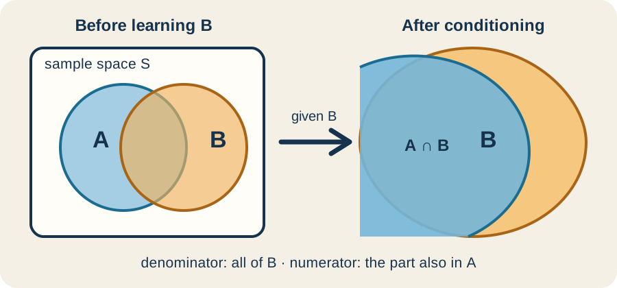
The restriction idea works whether outcomes are equally likely or not. Counting is convenient for cards, dice, and finite tables, but probability mass can also be unequal or continuous. In every case, the denominator must represent all probability still under consideration after the condition is known. The numerator must represent the probability that satisfies both the target and the condition. That invariant meaning is more reliable than any particular computational shortcut.

Derive and interpret the conditional-probability formula

For an event $B$ with positive probability, conditional probability is defined by $P(A\mid B)=\frac{P(A\cap B)}{P(B)}$. The expression is read as the probability of $A$ given $B$. The vertical bar $\mid$ is not division and does not mean “such that” in this context. It announces that $B$ is being treated as the reference space. The requirement $P(B)>0$ matters because dividing by zero cannot produce a probability distribution. Every symbol in the formula therefore records a specific part of the restriction process.

The denominator $P(B)$ rescales the surviving probability mass so that the new sample space has total probability one. The numerator $P(A\cap B)$ selects the part of that surviving mass that also belongs to $A$. Because $A\cap B$ is a subset of $B$, its probability cannot exceed $P(B)$. Consequently, the quotient always lies between zero and one when the probability model is valid. This range check is a quick way to detect an inverted fraction or an incorrect denominator.

Consider a class of $30$ students containing $18$ students who take chemistry, $12$ who take physics, and $8$ who take both. If one student is chosen and you learn that the student takes physics, then $B$ is the group of $12$ physics students. The target $A$ is taking chemistry, and the overlap contains $8$ students. Thus $P(A\mid B)=\frac{8/30}{12/30}=\frac{8}{12}=\frac{2}{3}$. The factors of $30$ cancel because conditioning replaces the original class with the physics subgroup.

Read the order of the notation carefully

Conditional probability is directional, so $P(A\mid B)$ and $P(B\mid A)$ usually describe different questions. In the class example, $P(\text{chemistry}\mid\text{physics})=\frac{8}{12}$ because twelve students satisfy the condition. Reversing the order gives $P(\text{physics}\mid\text{chemistry})=\frac{8}{18}$ because eighteen students now satisfy the condition. The same overlap appears in both numerators, but the reference groups differ. Reading the notation from left to right as “target given condition” makes that difference explicit.

Natural language can hide this order, especially in medical, legal, and engineering contexts. “The probability of a defect given alarm” asks what fraction of alarms correspond to defects. “The probability of an alarm given defect” asks how frequently the system detects an actual defect. The first quantity concerns the credibility of an alarm, while the second concerns detection sensitivity. Treating them as interchangeable is sometimes called the inverse fallacy.

A useful translation routine has three steps. First, underline the information introduced by words such as “given,” “among,” “of those,” or “provided that.” Second, place that event to the right of the vertical bar because it defines the denominator. Third, place the requested event to the left and form the intersection in the numerator. This routine turns a linguistic problem into a probability structure before numbers can distract you. It should become a deliberate habit whenever conditional language appears.

Build the multiplication rule from the definition

Starting with $P(A\mid B)=\frac{P(A\cap B)}{P(B)}$, multiply both sides by $P(B)$. The result is $P(A\cap B)=P(A\mid B)P(B)$. This multiplication rule says that the probability of following the $B$ branch and then reaching $A$ equals the probability of entering $B$ times the conditional probability of $A$ within $B$. The rule does not assume that $A$ and $B$ are independent. In fact, the conditional factor is precisely what allows the rule to represent dependence.

The intersection is symmetric, meaning $A\cap B=B\cap A$, so the same probability can be factored in the reverse order. Therefore $P(A\cap B)=P(B\mid A)P(A)$ as well. Equating the two factorizations gives $P(A\mid B)P(B)=P(B\mid A)P(A)$. This equality is the algebraic core of Bayes’ theorem. It also shows why reversing a conditional probability requires both events’ base probabilities.

The rule extends to a sequence through repeated conditioning. For three events, $P(A\cap B\cap C)=P(A)P(B\mid A)P(C\mid A\cap B)$. Each factor describes the next event under all information accumulated earlier along the path. Probability trees encode exactly this sequence, with multiplication along a single path. Adding across mutually exclusive completed paths then combines different ways the target event can occur.

Use tables and trees as reasoning tools

A two-way table makes conditional denominators visible by organizing counts across two categorical variables. To condition on a row category, divide the desired cell by that row total. To condition on a column category, divide the desired cell by that column total. The grand total is used only for an unconditional probability. Writing the relevant total beside the vertical bar helps keep the reference group fixed.

A probability tree emphasizes temporal or logical stages instead of rectangular counts. Branches leaving the same node must sum to one because they represent all possibilities under the information at that node. Multiply branch probabilities along a path to obtain the probability of the corresponding intersection. Add path probabilities only when those paths are mutually exclusive ways to reach the event of interest. The diagram below shows how the table and tree express the same joint structure.

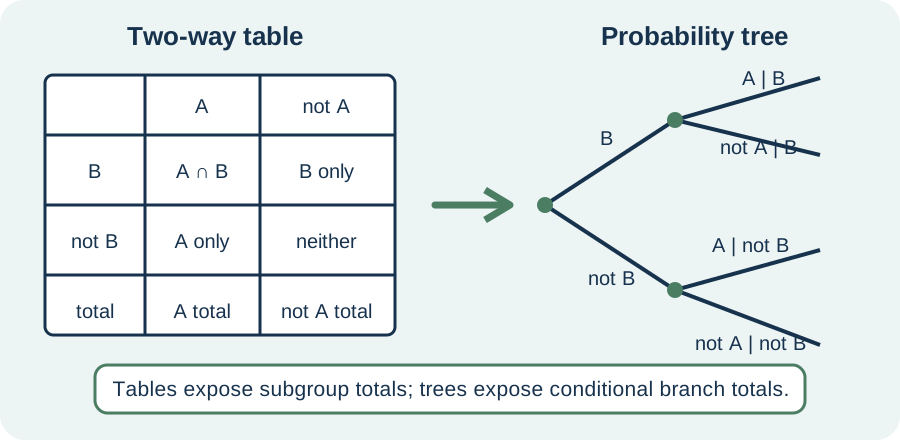
Choose the representation that makes the hidden denominator easiest to see. Tables are especially effective when actual frequencies are available or when two categories are crossed. Trees are especially effective for sequential events, repeated trials with changing probabilities, and diagnostic pathways. A Venn-style area diagram emphasizes intersections and restricted spaces but may not preserve exact proportions. Moving among representations is a form of verification because each one exposes different mistakes.

Distinguish independence from disjointness

Events $A$ and $B$ are independent when learning that one occurred does not change the probability of the other. In symbols, independence means $P(A\mid B)=P(A)$ whenever $P(B)>0$. Substituting the conditional definition gives the equivalent multiplication test $P(A\cap B)=P(A)P(B)$. The word “equivalent” means either equation can be used to establish the same relationship under the stated conditions. Independence is therefore a statement about information, not simply about whether two events look unrelated.

Disjoint events have no common outcomes, so $A\cap B=\varnothing$ and $P(A\cap B)=0$. If both disjoint events have positive probability, then learning that $B$ occurred forces the probability of $A$ to zero. Because that updated value differs from the original positive value, the events are dependent. Thus disjointness and independence are nearly opposites for nontrivial events. Confusing them often comes from using the informal word “separate” without specifying its mathematical meaning.

Suppose a fair six-sided die is rolled, with $A$ meaning “the result is even” and $B$ meaning “the result exceeds three.” Here $P(A)=\frac{3}{6}$, $P(B)=\frac{3}{6}$, and $P(A\cap B)=\frac{2}{6}$ because four and six satisfy both. The product $P(A)P(B)=\frac{1}{4}$ does not equal $\frac{1}{3}$, so the events are dependent. Equivalently, $P(A\mid B)=\frac{2}{3}$ differs from $P(A)=\frac{1}{2}$. A verbal impression cannot replace this explicit comparison. Both valid tests lead to the same conclusion.

Combine cases with the law of total probability

A collection of events $B_1,B_2,\ldots,B_n$ forms a partition when the events are mutually exclusive and together cover the entire sample space. Every outcome then belongs to exactly one partition category. Event $A$ can be divided into the disjoint pieces $A\cap B_1,A\cap B_2,\ldots,A\cap B_n$. Adding their probabilities and applying the multiplication rule gives $P(A)=\sum_{i=1}^{n}P(A\mid B_i)P(B_i)$. The sigma symbol $\sum$ means to add one term for every index $i$ from one through $n$.

Suppose a factory obtains $60\%$ of its parts from line 1 and $40\%$ from line 2. The defect rates are $2\%$ and $5\%$, respectively. The overall defect probability is $P(D)=(0.02)(0.60)+(0.05)(0.40)=0.032$. The result $0.032$ is equivalent to $3.2\%$. It is a weighted average because each conditional defect rate is weighted by its line’s share of production.

The weights must refer to the same population and must sum to one. Simply averaging $2\%$ and $5\%$ would incorrectly treat the two production lines as equally common. A total-probability calculation preserves both within-group behavior and group prevalence. This separation is essential whenever rates differ across hospitals, schools, machines, or demographic groups. Ask for the rate inside each case and the prevalence of each case. Both questions are necessary for the overall rate.

Reverse a condition with Bayes’ theorem

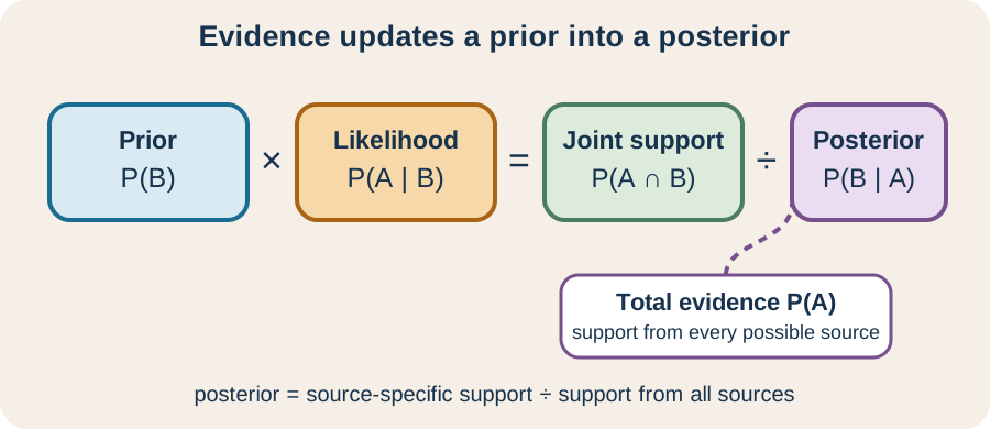
Bayes’ theorem follows by solving the equality $P(A\mid B)P(B)=P(B\mid A)P(A)$ for the desired conditional probability. The result is $P(B\mid A)=\frac{P(A\mid B)P(B)}{P(A)}$, provided $P(A)>0$. The numerator is the joint probability that both $B$ and $A$ occur. The denominator is the total probability of the observed evidence $A$. The quotient therefore asks what fraction of all evidence-producing cases came from source $B$.

When $B_1,\ldots,B_n$ partition the possible sources, substitute the law of total probability into the denominator. This produces $P(B_j\mid A)=\frac{P(A\mid B_j)P(B_j)}{\sum_{i=1}^{n}P(A\mid B_i)P(B_i)}$. The symbol $B_j$ marks the particular source being evaluated, while the index $i$ runs across every possible source in the denominator. The numerator supports one explanation of the evidence, and the denominator represents all explanations included in the model. Bayes’ theorem is consequently normalized comparison, not a mysterious reversal trick.

The diagram below organizes the update into prior, likelihood, evidence, and posterior. The prior $P(B)$ represents belief or prevalence before observing $A$. The likelihood $P(A\mid B)$ measures how compatible the evidence is with source $B$. The evidence $P(A)$ normalizes all source-weighted likelihoods. The posterior $P(B\mid A)$ is the updated probability after the evidence is included.

Understand base rates through natural frequencies

Consider a condition present in $1.0\%$ of a population, a test with $95\%$ sensitivity, and a $5.0\%$ false-positive rate. Sensitivity is $P(+\mid C)=0.95$, where $C$ denotes having the condition. The false-positive rate is $P(+\mid C^{c})=0.05$, where the superscript $c$ denotes the complement, or not having the condition. The desired probability after a positive result is $P(C\mid +)$, which reverses the stated sensitivity. A low prevalence can make this posterior much smaller than intuition expects.

Natural frequencies make the calculation concrete by imagining $10{,}000$ representative people. About $100$ have the condition, and $95$ of them test positive. About $9{,}900$ do not have the condition, and $495$ of them test positive. There are therefore $590$ positive tests in total, of which $95$ are true positives. The conditional probability is $P(C\mid +)=\frac{95}{590}\approx0.161$, or approximately $16.1\%$.

This result does not mean the test is useless or inaccurate. It means that false positives drawn from a large unaffected group can outnumber true positives drawn from a small affected group. The prevalence $P(C)$ is called a base rate because it describes how common the condition was before testing. Ignoring that rate creates the base-rate fallacy. Decisions should also consider consequences, follow-up tests, and uncertainty in the stated rates, which probability alone does not determine.

Check units, complements, and numerical meaning

Probabilities are dimensionless ratios, so they do not carry physical units such as meters or seconds. Counts used to form a probability must nevertheless refer to compatible units of observation, such as students out of students or defective parts out of inspected parts. Dividing eight chemistry-and-physics students by twelve physics students cancels the student count and leaves a pure ratio. Percentages are another notation for such ratios, with $16.1\%=\frac{16.1}{100}=0.161$. Keeping counts labeled until the final division makes the reference population clear.

Complements provide useful checks because $P(A^{c}\mid B)=1-P(A\mid B)$. Within any fixed condition $B$, the target event and its complement exhaust the restricted sample space. Similarly, conditional branches leaving the same tree node must sum to one. If a sensitivity is $0.95$, then the false-negative rate under the condition is $0.05$. This complement is different from the false-positive rate because the two rates condition on different populations.

A defensible final statement should name the condition, target, denominator, and interpretation. Instead of writing only $0.25$, say that among outcomes in $B$, one quarter also belong to $A$. Then confirm that the result lies between zero and one and is reasonable relative to the unrestricted probability. If the conditional value rises, the new information favors the target; if it falls, the information weighs against it. These verbal checks turn a calculation into an explanation. They also make an incorrect reference population easier to notice.

Diagnose common mistakes deliberately

The most common mistake is reversing $P(A\mid B)$ and $P(B\mid A)$. Prevent it by identifying the restricted group before inserting any numbers. A second mistake is using the grand total as the denominator even after the phrase “given that” has narrowed the population. A third is multiplying $P(A)P(B)$ without either establishing independence or using a conditional factor. Each error changes the probability model, not merely the arithmetic.

Another mistake is dividing by an event with zero probability. In an elementary discrete model, conditioning on an impossible event is undefined because there is no restricted population to normalize. More advanced probability theory can define conditional structures for continuous variables, but it does not repair ordinary division by zero. State the condition $P(B)>0$ when using the elementary definition. Domain restrictions are part of the theorem and should not be hidden.

Finally, avoid treating a model’s categories and rates as unquestionable facts. A Bayes calculation is only as appropriate as its partition, likelihoods, and prior information. Selection bias can make observed frequencies unrepresentative, and dependence between repeated observations can invalidate a simple product. Report assumptions alongside results, especially in health, safety, and policy applications. Mathematical precision includes being explicit about what the model leaves out.

Practice with retrieval, representation, and explanation

First, let $P(A)=0.50$, $P(B)=0.40$, and $P(A\cap B)=0.10$. Calculate $P(A\mid B)$ and decide whether $A$ and $B$ are independent. Then calculate $P(B\mid A)$ and explain why it differs from the first conditional probability. Your response should identify both denominators rather than giving numbers alone. Check independence using both the conditional and product criteria.

Second, return to the factory with production shares $60\%$ and $40\%$ and defect rates $2\%$ and $5\%$. Draw a two-stage tree, label every branch, and verify that all terminal path probabilities sum to one. Find the overall defect probability using total probability. Then find the probability that a defective part came from line 2 by applying Bayes’ theorem. Interpret the posterior as a fraction of all defective parts, not of all manufactured parts.

Third, design a small two-way table about two school activities with at least $40$ students. Choose counts so the two events are dependent but not disjoint. Compute both conditional directions, the intersection, and the product of the marginal probabilities. Explain how the table reveals dependence and how changing one cell could produce independence. Creating a valid example requires deeper control than merely recognizing one.

Solutions and checks

For the first problem, $P(A\mid B)=\frac{0.10}{0.40}=0.25$, which differs from $P(A)=0.50$, so the events are not independent. Also, $P(B\mid A)=\frac{0.10}{0.50}=0.20$ because the denominator changes when the condition changes. The product test agrees because $P(A)P(B)=(0.50)(0.40)=0.20$, not $0.10$. The intersection is too small for independence. Both conditional directions should be reported distinctly.

For the factory, the defective paths have probabilities $(0.60)(0.02)=0.012$ and $(0.40)(0.05)=0.020$. Adding them gives $P(D)=0.032$, or $3.2\%$. Bayes’ theorem then gives $P(\text{line 2}\mid D)=\frac{0.020}{0.032}=0.625$, or $62.5\%$. Line 2 supplies fewer parts but more defective parts. The posterior therefore exceeds its $40\%$ production share.

The third problem has many correct constructions. Verify that all four interior counts are nonnegative, row and column totals agree with the grand total, and neither event is empty. Dependence is shown when $P(A\mid B)\ne P(A)$ or, equivalently, when $P(A\cap B)\ne P(A)P(B)$. A complete explanation must specify which table total serves as each denominator. Recalculate all marginal totals after changing a cell.

Connect conditional probability to what comes next

Conditional probability becomes more powerful when outcomes are assigned numerical values through random variables. A conditional distribution describes how the entire distribution of a variable changes after information is observed. Conditional expectation then summarizes an updated distribution with a probability-weighted average. These ideas support regression, Markov chains, Bayesian inference, and stochastic processes. The restricted-sample-space principle remains unchanged even when the notation becomes more advanced.

Statistical inference also distinguishes probabilities about data under a model from probabilities assigned to hypotheses or parameters. Bayes’ theorem can connect these quantities only after a prior model and likelihood have been specified. Frequentist procedures use conditional reasoning too, although they interpret probability differently. Learning to name the random event and condition now will prevent serious confusion later. Notation is most useful when every symbol has a clear referent in the underlying experiment.

The durable lesson is that information changes the denominator before it changes the answer. Begin with the new reference group, locate the target within it, and only then compute. Use tables, trees, and natural frequencies to make that structure visible. Verify the result through range, complement, and representation checks. Conditional probability then becomes a disciplined method for learning from evidence rather than a collection of disconnected formulas.