Sample Spaces and Events

Probability begins by describing what could happen before assigning numerical weights. A sample space records possible outcomes, while events collect outcomes relevant to a question. Set notation turns words such as “or,” “and,” and “not” into operations that can be checked. The probability axioms constrain every valid assignment of weights. This lesson develops those ideas through models, diagrams, calculations, and deliberate error checks.

Begin with an experiment and its resolution

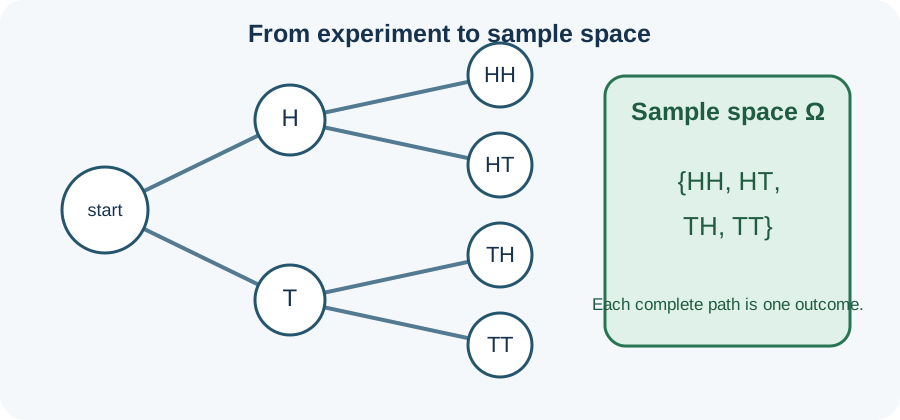
An experiment is a repeatable or conceptually repeatable process whose result is uncertain. A single performance of that process is called a trial. An outcome records what happened on one trial at the detail level chosen by the modeler. The sample space, written $\Omega$, is the set containing every outcome the model permits. The Greek capital letter omega is conventional, but its meaning comes from the stated definition.

The required resolution depends on the question. For two coin tosses, $\Omega=\{HH,HT,TH,TT\}$ preserves order, where $H$ means heads and $T$ means tails. If the question asks for the number of heads, one can later map these four outcomes to $0$, $1$, or $2$. Beginning with only $\{0,1,2\}$ can hide that the middle value arises in two different ways. A useful space retains every distinction needed by later events and probability assignments.

A model also states what it deliberately ignores. A physical coin has an orientation, landing position, and microscopic trajectory that an elementary model omits. That simplification is acceptable when those details do not affect the question or assumed probabilities. It is not acceptable to omit an inconvenient result that the experiment can produce. Before calculating, verify that outcomes are exhaustive, distinguishable, and defined at one consistent resolution.

Distinguish outcomes from events

An elementary outcome is one member $\omega$ of the sample space $\Omega$. The lowercase omega represents a particular result, while capital omega represents the complete set. An event $A$ is a subset of $\Omega$, written $A\subseteq\Omega$. The event occurs when the observed outcome belongs to that subset. Events are therefore propositions that become true or false after an outcome is observed.

For a six-sided die, use $\Omega=\{1,2,3,4,5,6\}$. The event “an even result” is $E=\{2,4,6\}$. The event “the result exceeds four” is $G=\{5,6\}$. If the die shows $6$, both $E$ and $G$ occur even though only one elementary outcome occurs. Different event names do not imply that the events are mutually exclusive.

The whole sample space is the certain event because every allowed outcome belongs to it. The empty set $\varnothing$ is the impossible event because it contains no outcomes. These labels are relative to the adopted model rather than claims that the model includes every physical detail. An event may contain one outcome, many outcomes, all outcomes, or none. Keeping outcome and event language separate prevents confusion in later formulas.

Translate logical language into set operations

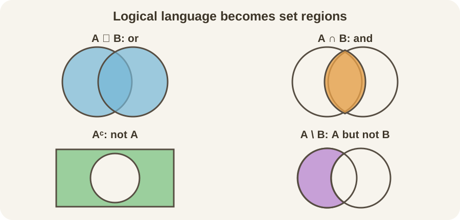
The union $A\cup B$ contains outcomes belonging to $A$, to $B$, or to both. The symbol $\cup$ visually suggests combining two containers. In probability language, union corresponds to the inclusive word “or.” Unless a problem explicitly excludes the overlap, shared outcomes remain in the union. Writing event sets before calculating makes this convention visible. The union is itself another event inside the same sample space.

The intersection $A\cap B$ contains outcomes belonging to both events. The symbol $\cap$ marks the portion shared by the two sets. Intersection corresponds to the logical word “and.” For $E=\{2,4,6\}$ and $G=\{5,6\}$, the intersection is $E\cap G=\{6\}$. A nonempty intersection means the events can occur together on one trial. Intersection therefore answers a simultaneous-condition question.

The complement $A^c$ contains every outcome in $\Omega$ that is not in $A$. The superscript $c$ means complement and is not an exponent. The difference $A\setminus B$ contains outcomes in $A$ but not in $B$. Parentheses in compound expressions specify which set operation is performed first. Translating one phrase at a time reduces logical errors before numbers enter the reasoning.

Identify disjoint, exhaustive, and partitioned events

Events $A$ and $B$ are disjoint when $A\cap B=\varnothing$. This equation says that no outcome belongs to both events. Disjoint events cannot occur during the same trial. The phrases disjoint and mutually exclusive mean the same thing here. They do not mean that the events have equal probabilities or influence one another.

A collection is exhaustive when the union of its events equals the sample space. For a die, the events “odd” and “even” are both disjoint and exhaustive. The events “less than four” and “greater than four” are disjoint but not exhaustive because outcome $4$ is missing. Checking both properties is useful when constructing cases. A partition is a collection of nonempty events that is pairwise disjoint and exhaustive.

Partitions organize complicated questions without double counting. If $A_1,A_2,\ldots,A_n$ partition $Omega$, exactly one $A_i$ occurs on each trial. The subscript $i$ labels a case and does not indicate multiplication. Later, conditional probability uses partitions to combine case-specific calculations. For now, verify every intersection and the complete union instead of trusting a verbal list.

Build probability from three axioms

A probability measure $P$ assigns a number $P(A)$ to each event $A$. The first axiom requires $P(A)\geq0$, so probability cannot be negative. The second requires $P(\Omega)=1$, which normalizes certainty to one. A probability can become a percentage by multiplying it by $100\%$. Probability is dimensionless because it is a proportion rather than a physical measurement.

The third axiom says that probabilities add across disjoint events. When $A\cap B=\varnothing$, it gives $P(A\cup B)=P(A)+P(B)$. The principle extends to any finite collection of pairwise disjoint events. This rule connects the geometry of sets with arithmetic. Its disjointness condition matters because shared outcomes would otherwise be counted repeatedly.

Many familiar rules follow from these axioms. Every event lies within $Omega$, so its probability cannot exceed one. The empty set has probability zero because adding it to a disjoint event changes nothing. An event and its complement divide all probability mass between them. Derived formulas should be understood through these structural facts rather than memorized as isolated tricks.

Derive complement and addition rules

An event and its complement partition the sample space. Symbolically, $A\cap A^c=\varnothing$ and $A\cup A^c=\Omega$. Additivity gives $P(A)+P(A^c)=P(\Omega)=1$. Solving for the complement produces $P(A^c)=1-P(A)$. The subtraction represents all probability mass remaining outside event $A$.

Complement reasoning is efficient for “at least one” questions. If a fair coin is tossed four independent times, let $A$ mean at least one head. Its complement means four tails, with probability $\left(\dfrac{1}{2}\right)^4=\dfrac{1}{16}$. Thus $P(A)=1-\dfrac{1}{16}=\dfrac{15}{16}$. State the complement in words before subtracting to avoid reversing the intended event.

Overlapping events require the general addition rule $P(A\cup B)=P(A)+P(B)-P(A\cap B)$. Adding the first two probabilities counts their shared region twice. Subtracting the intersection removes one duplicate copy. If the events are disjoint, the intersection probability is zero and the rule reduces to ordinary addition. A Venn diagram makes every term correspond to a visible region.

Use equal likelihood only when justified

For a finite space containing $N$ equally likely outcomes, an event with $m$ outcomes has probability $P(A)=\dfrac{m}{N}$. The numerator counts favorable outcomes, and the denominator counts all possible outcomes. The horizontal fraction bar means division of the entire numerator by the entire denominator. This formula follows from equal weights and additivity. It is not a universal definition of probability.

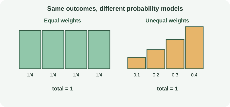
A fair die supports weight $\dfrac{1}{6}$ for each of its six faces. A loaded die can use the same sample space while assigning different face probabilities. Counting three even faces does not establish probability one-half for that loaded die. Physical symmetry, calibration, or an explicit assumption must justify equal likelihood. Similar-looking labels alone provide no such justification.

Grouped categories can also destroy equal likelihood. The counts $0$, $1$, and $2$ heads in two fair tosses are not equally probable. Their probabilities are $\dfrac{1}{4}$, $\dfrac{2}{4}$, and $\dfrac{1}{4}$ because one head has two underlying sequences. Returning to $\{HH,HT,TH,TT\}$ reveals those multiplicities. Uniform elementary outcomes need not remain uniform after grouping.

Construct sample spaces with trees and counting

A tree diagram represents an experiment occurring in stages. Every path from the root to an endpoint corresponds to one elementary outcome. Branch labels may record probabilities at each stage. Multiplying appropriate branch probabilities gives a path probability when the model supports that conditional product. Adding endpoint probabilities should return one and thereby check completeness.

The multiplication principle counts successive choices. If one stage has $m$ options and every such choice leads to $n$ options, there are $mn$ ordered outcomes. Each first-stage option pairs with every compatible second-stage option. Additional stages contribute additional factors. Write what each factor counts so a bare product never replaces the modeling argument.

Counting does not automatically produce probability. A count answers how many outcomes satisfy structural rules. A probability ratio also needs equal likelihood or explicit outcome weights. Human-selected passwords, for example, are rarely uniform even when many strings are technically available. Keep the combinatorial question “how many?” separate from the probabilistic question “how likely?” This separation prevents a correct count from supporting an unjustified probability.

Compare ordered and unordered selections

A permutation counts an ordered selection. Choosing $r$ distinct objects from $n$ without replacement gives $P(n,r)=\dfrac{n!}{(n-r)!}$. The exclamation mark denotes factorial, with $n!=n(n-1)\cdots2\cdot1$. The denominator cancels unused factors from the full factorial. This formula condenses a descending multiplication-principle product.

A combination counts a selection for which order does not matter. Its formula is $\binom{n}{r}=\dfrac{n!}{r!(n-r)!}$, read “$n$ choose $r$.” Division by $r!$ removes the different orderings of each selected group. Whether order matters comes from the outcome definition. It must not be decided merely by which formula is remembered first. Listing a tiny example often reveals whether reordered selections remain distinct.

Choosing a president and treasurer from ten students is ordered because the offices differ. Choosing two identical-role representatives from ten students is unordered. The first task has $10\cdot9=90$ outcomes, while the second has $\binom{10}{2}=45$. Every unordered pair appears twice in the ordered count. Explaining that factor of two connects the two formulas conceptually.

Work with unequally weighted outcomes

Finite outcomes may receive unequal weights. Assign weight $p_i$ to outcome $\omega_i$, with $p_i\geq0$ and $\sum_i p_i=1$. The subscript $i$ simply identifies an outcome in the list. An event probability is the sum of weights belonging to its outcomes. This construction automatically satisfies all three probability axioms.

Suppose a loaded die has probabilities $\dfrac{1}{10},\dfrac{1}{10},\dfrac{1}{10},\dfrac{2}{10},\dfrac{2}{10},\dfrac{3}{10}$ for faces one through six. The weights are nonnegative and sum to one. The probability of an even result is $\dfrac{1}{10}+\dfrac{2}{10}+\dfrac{3}{10}=\dfrac{6}{10}=\dfrac{3}{5}$. Counting even faces would instead give the incorrect value one-half. Weighted addition respects the stated model.

Weights can arise from theory, calibration data, repeated observations, or a reasoned uncertainty model. Mathematics alone does not decide which source is appropriate. It determines whether assignments remain coherent after they are chosen. A solution should distinguish modeling assumptions from deductions. Stating where weights came from is part of communicating a probability result responsibly.

Solve an integrated two-dice example

Two fair six-sided dice are rolled, and ordered pair $(i,j)$ records their results. The sample space contains $6\cdot6=36$ equally likely outcomes. Parentheses identify an ordered pair, so $(2,5)$ differs from $(5,2)$. Let $A$ mean that the sum is seven. Six pairs satisfy that condition, so $P(A)=\dfrac{6}{36}=\dfrac{1}{6}$.

Let $B$ mean that at least one die shows six. Six outcomes have first coordinate six, and six have second coordinate six. The pair $(6,6)$ belongs to both groups and must appear only once in the union. Thus $B$ has $6+6-1=11$ outcomes. Equal likelihood gives $P(B)=\dfrac{11}{36}$.

The intersection $A\cap B$ contains $(1,6)$ and $(6,1)$, so its probability is $\dfrac{2}{36}$. Inclusion–exclusion gives $P(A\cup B)=\dfrac{6}{36}+\dfrac{11}{36}-\dfrac{2}{36}=\dfrac{15}{36}=\dfrac{5}{12}$. Every denominator refers to the same 36-outcome space. Listing the intersection explains exactly why two outcomes are subtracted. Agreement between listing and algebra is a valuable independent check.

Diagnose errors and practice deliberately

An incomplete sample space is a frequent modeling failure. Ties, repeated values, boundary cases, or unusual results may be omitted. Ask what every possible trial would be called. If a result has no label, the space is incomplete. If one result receives two elementary labels at the same resolution, the categories overlap.

Another error is confusing disjointness with independence. Disjoint nonempty events cannot occur together, whereas independent events do not change one another’s probabilities. Those ideas are generally very different. This lesson uses disjointness to justify addition. Independence belongs to later work involving products and conditional probability.

Practice by constructing the ordered sample space for three coin tosses. Let $A$ mean exactly two heads and $B$ mean a head on the first toss. Find the two event sets, their intersection, and their union before calculating probabilities. Check the union by direct counting and by the addition rule. Explain exactly where fairness and independence enter the model.

Connect forward to conditional probability

Events provide the language for representing new information. If evidence says event $B$ occurred, a later lesson will restrict attention to outcomes inside $B$. Conditional probability then renormalizes weights within that reduced space. The expression $P(A\mid B)$ reads “probability of $A$ given $B$.” Its vertical bar separates the target event from the stated condition. The notation makes the information state visible inside the probability statement.

Random variables will map outcomes to numerical values. Several elementary outcomes can produce the same numerical value, so their probabilities must be combined. The distinctions among outcomes, events, and values remain essential. Distributions and expectations inherit coherence from the underlying event structure. Sophisticated calculations cannot rescue an inconsistent sample-space model.

You are prepared to continue when you can move among words, sets, diagrams, and probabilities without changing the modeled event. You should justify equal likelihood, identify overlap, and explain every numerator and denominator. You should also recognize when a counting result is not yet a probability. Those habits turn probability from formula selection into disciplined modeling. Conditional probability can then build on a stable foundation.