Polynomial Operations

A polynomial is a finite sum of power terms, but that short definition hides an unusually rich structure. Addition aligns like powers, multiplication distributes every term, and division reverses multiplication while tracking a remainder. The same exponent laws used in elementary algebra explain each operation. Degree and leading coefficient then predict how the expression behaves for large inputs. Learning the structure makes polynomial arithmetic easier to reconstruct and verify than a collection of memorized tricks.

Polynomials appear whenever a changing quantity is approximated by powers of an input. Position models, area formulas, cost functions, and Taylor approximations all use them. Correct manipulation therefore supports later work in functions, calculus, physics, and numerical methods. This lesson develops meaning before speed, then introduces reliable workflows for efficient calculation. Each workflow includes prediction checks so that an answer can be evaluated before it is trusted.

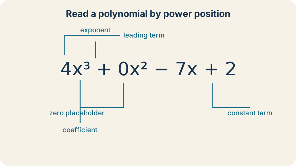
Standard form places powers in descending order. Each coefficient multiplies one power of the variable. A missing power has coefficient zero even when it is not written. The leading term controls degree and large-input behavior. Constant terms occupy the power-zero position because $x^0=1$ for nonzero $x$.

Recognize polynomial structure

A polynomial in $x$ has the form $P(x)=a_nx^n+a_{n-1}x^{n-1}+\cdots+a_1x+a_0$. The symbol $P$ names the polynomial function, while $P(x)$ denotes its value at input $x$. Each $a_k$ is a coefficient and each exponent $k$ is a nonnegative integer. The sum is finite, so it ends after a definite number of terms. If $a_n\ne0$, the degree is $n$ and the leading coefficient is $a_n$.

A term is a coefficient multiplied by a nonnegative integer power of the variable. In $4x^3-7x+2$, the terms are $4x^3$, $-7x$, and $2$. The constant $2$ can be viewed as $2x^0$. The missing $x^2$ term has coefficient zero. Recognizing that hidden placeholder becomes important during subtraction and long division.

Expressions containing $x^{-1}$, $\sqrt{x}=x^{\frac{1}{2}}$, or a variable in a denominator are not polynomials in $x$. An infinitely continuing power series is also not a polynomial because it has infinitely many terms. Coefficients may be negative, fractional, irrational, or complex without violating the definition. It is the exponents and finiteness that determine polynomial status. Classification should therefore inspect structure rather than visual complexity.

Interpret degree and leading terms

Degree measures the highest power with a nonzero coefficient. The polynomial $-3x^5+2x^2-7$ has degree $5$ and leading coefficient $-3$. Its leading term is $-3x^5$. Lower-degree terms may matter greatly near particular inputs and zeros. For sufficiently large $|x|$, however, the leading term dominates their relative size.

The parity of the degree and sign of the leading coefficient predict end behavior. Even-degree polynomials have matching left and right directions because $x^n$ is positive at both ends when $n$ is even. Odd-degree polynomials have opposite directions because $x^n$ changes sign when $x$ changes sign. A positive leading coefficient preserves those base directions, while a negative coefficient reverses them. Thus $-3x^5+2x^2-7$ rises to the left and falls to the right.

Degree is not defined for the zero polynomial in the same ordinary way because every coefficient is zero. This special case prevents false statements about cancellation. For nonzero polynomials, $\deg(PQ)=\deg P+\deg Q$. For sums, degree is at most the larger input degree because leading terms may cancel. Predicting degree before calculating provides a useful error check.

Add by aligning like powers

Like terms contain exactly the same variable raised to exactly the same power. They can be combined because distribution gives $ax^k+bx^k=(a+b)x^k$. Terms such as $3x^2$ and $-5x^2$ are like terms, whereas $3x^2$ and $3x^3$ are not. Their powers represent different functions of $x$. Adding polynomials therefore means adding coefficient values within matching power positions.

Consider $(3x^3-2x+5)+(x^3+4x^2-7)$. Write the first polynomial as $3x^3+0x^2-2x+5$ to expose its missing quadratic term. Then add coefficients by columns: $3+1=4$, $0+4=4$, $-2+0=-2$, and $5-7=-2$. The result is $4x^3+4x^2-2x-2$. Its degree $3$ agrees with the predicted maximum degree.

This operation resembles addition by place value. One would not add tens to hundreds merely because both are digits. Likewise, one does not combine $x^2$ with $x^3$ merely because both involve $x$. Standard form makes the alignment visible. A quick numerical check at a simple input such as $x=1$ can confirm that the original sum and simplified result agree.

Subtract by distributing the negative

Subtraction means adding the opposite of the entire second polynomial. In symbols, $P(x)-Q(x)=P(x)+[-Q(x)]$. Every coefficient of $Q$ must change sign, including coefficients not immediately next to a subtraction mark. Parentheses protect the scope of the operation. Removing them without distributing the negative is one of the most common polynomial errors.

Simplify $(4x^2-x+3)-(x^2+5x-8)$. Distribute the negative to obtain $4x^2-x+3-x^2-5x+8$. Combining like terms gives $3x^2-6x+11$. Notice that subtracting the constant $-8$ produced $+8$. A sign-by-sign rewrite before combining reduces working-memory demands.

Evaluate both forms at $x=2$ as a check. The original expression gives $(16-2+3)-(4+10-8)=17-6=11$. The simplified expression gives $3(4)-6(2)+11=11$. Agreement at one input does not prove an identity, but disagreement would reveal an error. Structural derivation supplies the proof, while numerical substitution supplies a useful diagnostic.

Multiply through complete distribution

Multiplication uses the distributive law so that every term in one factor multiplies every term in the other. For monomials, multiply coefficients and add exponents of the same base. The exponent rule $x^a x^b=x^{a+b}$ explains why $2x^2\cdot3x^4=6x^6$. After all products are formed, like powers are combined. No separate trick is needed.

Expand $(x-3)(2x^2+x+4)$. Multiplication by $x$ gives $2x^3+x^2+4x$, while multiplication by $-3$ gives $-6x^2-3x-12$. Adding these rows produces $2x^3-5x^2+x-12$. The product degree is $1+2=3$, and the leading coefficient is $1\cdot2=2$. Both predictions match the expanded result.

The familiar FOIL acronym applies only to two binomials and can conceal the broader principle. A table or area model works for factors of any length. Row labels represent terms from one factor, column labels represent terms from the other, and each cell contains one product. Diagonals or matching-power groups are then combined. This representation makes omissions visible because every row–column pair requires a cell.

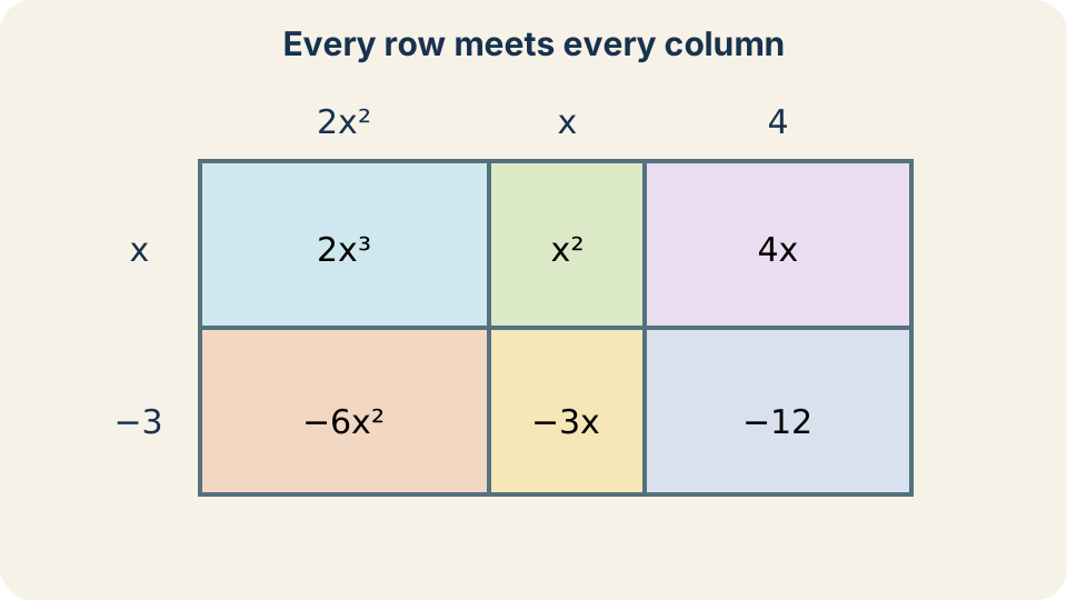
The multiplication grid is a visual form of distribution. Every row term meets every column term exactly once. Each cell records one coefficient product and one exponent sum. Cells with matching powers are combined after multiplication. The complete grid prevents missing cross terms. It works for polynomials with more than two terms.

Connect multiplication to geometric area

Suppose a rectangle has length $(x+5)\,\mathrm{m}$ and width $(x+2)\,\mathrm{m}$. Splitting each side at its constant part divides the rectangle into four smaller regions. Their areas are $x^2\,\mathrm{m}^2$, $5x\,\mathrm{m}^2$, $2x\,\mathrm{m}^2$, and $10\,\mathrm{m}^2$. Adding gives $(x^2+7x+10)\,\mathrm{m}^2$. This geometric decomposition is the distributive law made visible.

Units clarify why the terms can be added. If $x$ represents a length in metres, then the coefficients in expressions such as $x+5\,\mathrm{m}$ must be interpreted consistently. Every area contribution has square-metre units after multiplication. The term $7x$ inherits an implied metre coefficient so that it represents square metres in context. A physically meaningful sum requires every term to have identical dimensions.

The area model also explains factoring as reverse multiplication. If $x^2+7x+10$ is recognized as the sum of four rectangle pieces, the side lengths can be reconstructed as $x+5$ and $x+2$. Expansion moves from factors to a sum. Factoring moves from a sum to factors. Understanding this inverse relationship prepares later work with zeros and equations.

Divide by reversing multiplication

For polynomials $P$ and nonzero $D$, division seeks polynomials $Q$ and $R$ satisfying $P(x)=D(x)Q(x)+R(x)$ with $\deg R<\deg D$. The letters stand for dividend, divisor, quotient, and remainder. This equation is the polynomial analogue of integer division. The remainder condition guarantees that division cannot continue. If $R=0$, the divisor is an exact factor.

Long division works by canceling the current leading term. Divide the leading term of the remaining dividend by the leading term of the divisor to choose the next quotient term. Multiply the entire divisor by that term, subtract, and bring down the next power. Repeat until the remainder degree is smaller than the divisor degree. Zero-coefficient placeholders keep corresponding powers aligned throughout the process.

For example, divide $2x^3+3x^2-5x+6$ by $x+2$. Successive cancellation gives quotient $2x^2-x-3$ and remainder $12$. The result is verified by $2x^3+3x^2-5x+6=(x+2)(2x^2-x-3)+12$. Multiplying the divisor and quotient and then adding the remainder recovers the dividend. Verification reverses the operation and checks every coefficient simultaneously.

Use synthetic division when the divisor is linear

Synthetic division abbreviates long division for a divisor of the form $x-c$. The number used in the synthetic setup is $c$, not the visible constant with its original sign. Thus division by $x+2=x-(-2)$ uses $c=-2$. Only coefficients are written, and zeros must fill missing powers. The arithmetic reproduces repeated multiplication by $c$ and addition.

Divide $x^3+0x^2-4x+1$ by $x-2$. Synthetic steps with $2$ produce quotient coefficients $1,2,0$ and remainder $1$. Therefore $x^3-4x+1=(x-2)(x^2+2x)+1$. The zero coefficient in the quotient is normally omitted from its final form. Its placeholder was still necessary during the calculation.

Synthetic division is efficient but not more fundamental than long division. It relies on the special coefficient pattern of a monic linear divisor. For higher-degree divisors or divisors whose leading coefficient is not one, long division is usually clearer at this level. Choosing a method should follow from the divisor’s structure. Both methods must satisfy the same dividend-equals-divisor-times-quotient-plus-remainder identity.

Apply the Remainder and Factor Theorems

The Remainder Theorem states that division of $P(x)$ by $x-c$ leaves remainder $P(c)$. Substitute $x=c$ into $P(x)=(x-c)Q(x)+R$. The product $(c-c)Q(c)$ becomes zero, leaving $P(c)=R$. This short derivation explains the theorem rather than asking it to be memorized. Evaluation can therefore replace a full division when only the remainder is needed.

Let $P(x)=x^3+2x-5$ and divide conceptually by $x-2$. The remainder is $P(2)=2^3+2(2)-5=7$. No quotient calculation is necessary. If the result had been zero, $x-2$ would divide $P$ exactly. The theorem connects function values, division, and factors.

The Factor Theorem states that $x-c$ is a factor of $P(x)$ exactly when $P(c)=0$. The phrase “exactly when” expresses two directions. A factor produces zero upon substitution because one factor becomes $c-c=0$. Conversely, zero remainder means the division is exact and $x-c$ is a factor. This relationship later connects factors with graph intercepts and equation solutions.

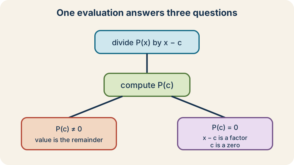
Dividing by $x-c$ produces the remainder $P(c)$. If that value is nonzero, it records what remains after division. If it equals zero, division is exact. Exact division makes $x-c$ a factor. The same condition makes $c$ a zero of the polynomial function. Evaluation therefore links three apparently different questions.

Track closure and degree

Polynomials are closed under addition, subtraction, and multiplication. Closure means that applying one of those operations to polynomials produces another polynomial. Coefficients may change and leading terms may cancel, but no forbidden exponent is introduced. Multiplication adds nonnegative integer exponents, which keeps them nonnegative integers. Finite sums and products also remain finite.

Division behaves differently. The quotient of two polynomials may be a rational expression rather than a polynomial. For example, dividing $1$ by $x$ produces $\frac{1}{x}=x^{-1}$, which is not a polynomial. Polynomial division instead reports a polynomial quotient plus a controlled remainder. Closure therefore depends on the operation being used.

Degree rules provide fast consistency checks. For nonzero products, degrees add because leading coefficients multiply to a nonzero value. For sums, degree cannot exceed the larger input degree, but it may fall when leading terms cancel. Division predicts $\deg Q=\deg P-\deg D$ when the dividend degree is at least the divisor degree and leading cancellation proceeds normally. These predictions can reveal an omitted term before detailed arithmetic is rechecked.

Distinguish identities from equations

An identity is true for every input in its domain. The statement $(x+1)^2=x^2+2x+1$ is an identity because complete distribution transforms one side into the other. The equals sign asserts two expressions name the same function. Substituting several values can support confidence but does not by itself prove universal equality. Algebraic transformation establishes the identity.

An equation such as $(x+1)^2=9$ is true only for particular inputs. Taking square roots gives $x+1=3$ or $x+1=-3$, so $x=2$ or $x=-4$. These values form the solution set. The equation does not permit replacing $(x+1)^2$ with $9$ in unrelated contexts. Its equality is conditional on the selected solutions.

Polynomial operations can prove identities or prepare equations for solving. Expansion may reveal that two formulas are identical. Factoring may expose values that make a product zero. Division can separate a known factor and lower the remaining degree. Before manipulating an equals sign, decide whether the task concerns equivalence for all inputs or truth at selected inputs.

Preserve units in polynomial models

Suppose position is $s(t)=a_2t^2+a_1t+a_0$, with $s$ measured in metres and $t$ in seconds. Every term in the sum must have metre units. Therefore $a_2$ has units $\frac{\mathrm{m}}{\mathrm{s}^2}$, $a_1$ has units $\frac{\mathrm{m}}{\mathrm{s}}$, and $a_0$ has units $\mathrm{m}$. Multiplication by the appropriate power of seconds converts each term to metres. Unlike dimensions would signal a malformed sum.

Coefficients are not always pure numbers. They can carry precisely the units needed to make terms comparable. In a cost model $C(q)=aq^2+bq+c$, the units of $a$ and $b$ depend on the units of quantity $q$ and cost $C$. If $q$ is items and $C$ is dollars, then $a$ has \frac{\}{\mathrm{item}^2}$and$b$has$\frac{$}{\mathrm{item}}$. Dimensional analysis therefore constrains possible coefficients.

Expanding a factored physical model must preserve units. A rectangle with sides $(x+2\,\mathrm{m})$ and $(x+5\,\mathrm{m})$ requires $x$ itself to represent a length. Every expanded term then has square-metre units. Writing bare constants without their contextual units may be convenient algebraically, but the interpretation should restore them. Unit awareness connects symbolic correctness with physical validity.

Use an error-resistant workflow

First rewrite every polynomial in descending powers and insert zero placeholders when alignment matters. Second predict the likely degree and leading coefficient of the result. Third perform exactly one operation at a time, keeping signs and parentheses visible. Fourth combine only like powers after all required distribution is complete. Finally verify through reverse operations, degree checks, or substitution at a simple input.

For multiplication, count the expected pairwise products before combining. A polynomial with three terms multiplied by one with two terms creates six raw products. For long division, multiply the completed quotient by the divisor and add the remainder. For subtraction, compare the rewritten signs with the original parentheses. These checks target the most common failure points rather than merely repeating the same arithmetic.

Speed should follow structure rather than replace it. Mental shortcuts are useful after the distributive reasoning is secure. If an answer’s degree contradicts the prediction, stop before moving onward. If a numerical check disagrees, compare the original and simplified values line by line. Self-correction is a mathematical skill, not evidence that the first attempt failed to count.

Practice and connect forward

Simplify $(4x^2-x+3)-(x^2+5x-8)$. Distributing the negative and combining aligned powers gives $3x^2-6x+11$. Expand $(2x+1)(x^2-3x+4)$ by complete distribution. The result is $2x^3-5x^2+5x+4$. Its cubic degree and leading coefficient $2$ agree with predictions.

For $P(x)=x^3+2x-5$, the remainder after division by $x-2$ is $P(2)=7$. For $x^3-4x+1$ divided by $x-2$, the quotient is $x^2+2x$ and the remainder is $1$. Multiplying gives $(x-2)(x^2+2x)+1=x^3-4x+1$. This reverse check confirms every coefficient. Evaluation at $x=2$ confirms the remainder independently.

Polynomial operations prepare several next ideas. Factoring reverses multiplication and exposes zeros. Graphing uses degree, leading terms, and zeros to predict shape. Rational functions use polynomial division to reveal asymptotes and remainders. Calculus later differentiates and integrates polynomials term by term because their power structure behaves so predictably.