Electronic Structure of Atoms

Atoms emit and absorb only particular colors of light. Those discrete spectral lines reveal that electron energy changes are quantized rather than continuously selectable. Modern atomic theory describes electrons with quantum states and wavefunctions. An orbital is a mathematical probability-amplitude pattern associated with an allowed state. It is not a miniature path around the nucleus.

The quantum model asks different questions from a planetary picture. It predicts probability distributions, energies, angular properties, and measurement outcomes rather than exact trajectories. Symbols such as $n$, $\ell$, $m_\ell$, and $m_s$ label allowed state properties. Their permitted values are constrained. Those constraints generate shells, subshells, orbitals, and electron capacities.

This lesson begins with spectroscopy because a model should answer evidence. Photon energy will connect line frequency with atomic energy differences. Wavefunctions and probability density will then establish the meaning of an orbital. Quantum numbers will organize states, and node patterns will connect mathematics with shape. The final sections will prepare for electron configurations without prematurely turning orbitals into rigid boxes.

Learning objectives and an opening prediction

After this lesson, you should use photon frequency or wavelength to calculate an atomic energy change. You should explain why line spectra support discrete energy states. You should distinguish a wavefunction from probability density and an orbital from a classical orbit. You should assign allowed quantum-number values and calculate subshell capacities. You should also relate nodes and orbital shapes while stating the model’s limits.

Imagine exciting a sample of hydrogen gas and observing it through a spectroscope. Predict whether the result is a continuous rainbow or isolated bright lines. Hydrogen produces discrete lines because only specific energy differences between allowed states occur. Each emitted photon carries one of those differences. The pattern acts like an atomic fingerprint.

Now imagine an electron drawn as a bead on a circular ring. That image may suggest a definite path, radius, and instantaneous location. The quantum orbital does not supply those classical quantities simultaneously. It supplies a state whose squared wavefunction predicts spatial detection probability. Replacing orbit with orbital requires changing the mental model, not just adding two letters.

Spectral lines are experimental evidence

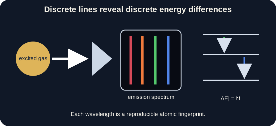
A low-density excited gas emits bright lines at characteristic wavelengths. A cool gas in front of a continuous light source can absorb corresponding wavelengths, producing dark lines. Each chemical element has a distinctive pattern because its allowed electronic states differ. Spectroscopy therefore identifies composition and probes energy structure. Astronomers can infer stellar elements without collecting a physical sample.

If electron energies were continuously available, isolated sharp transition lines would be difficult to explain. Instead, atoms exchange photons whose energies match differences between allowed states. The observed wavelengths are reproducible. Instrument resolution and physical broadening give lines finite width, but the central values remain structured. Quantization is an inference from this regular evidence.

Hydrogen’s relatively simple spectrum inspired early models, including Bohr’s quantized circular orbits. That model predicts hydrogen-like energies usefully but fails as a complete description of multi-electron atoms and detailed spectra. Quantum mechanics replaces classical paths with wavefunctions. Historical models remain helpful when their scope is stated. Scientific models evolve by explaining more evidence with fewer contradictions.

Photon energy connects light and atoms

A photon’s energy is $E_{\mathrm{photon}}=hf$. The symbol $h$ is Planck’s constant, approximately $6.626\times10^{-34}\,\mathrm{J\,s}$, and $f$ is frequency in hertz or inverse seconds. Multiplying joule-seconds by inverse seconds gives joules. Higher frequency means greater photon energy. One photon is absorbed or emitted per elementary transition event in the simple picture.

Because $c=\lambda f$ in vacuum, photon energy can also be written $E_{\mathrm{photon}}=\frac{hc}{\lambda}$. The symbol $c$ is vacuum light speed, approximately $3.00\times10^8\,\mathrm{\frac{m}{s}}$, and $\lambda$ is vacuum wavelength in meters. The horizontal fraction bar places the product $hc$ over the entire wavelength. Shorter wavelength means greater photon energy. Unit conversion from nanometers to meters is essential.

For an atomic transition, $|\Delta E_{\mathrm{atom}}|=hf$. If the atom drops from higher to lower energy, $\Delta E_{\mathrm{atom}}<0$ and a positive-energy photon is emitted. If the atom rises, it absorbs a photon and $\Delta E_{\mathrm{atom}}>0$. The absolute-value form gives photon-energy magnitude while words specify direction. Energy conservation connects the atom and radiation accounts.

Worked photon calculation

Consider a spectral line at $656.3\,\mathrm{nm}$. Convert wavelength to $656.3\times10^{-9}\,\mathrm m$. Photon energy is $E=\frac{(6.626\times10^{-34}\,\mathrm{J\,s})(2.998\times10^8\,\mathrm{\frac{m}{s}})}{656.3\times10^{-9}\,\mathrm m}$. Seconds and meters cancel through the fraction. The result is $3.027\times10^{-19}\,\mathrm J$ per photon.

Chemists often express photon energy per mole. Multiply by Avogadro’s constant: $(3.027\times10^{-19}\,\mathrm{\frac{J}{photon}})(6.022\times10^{23}\,\mathrm{\frac{photons}{mol}})=1.823\times10^5\,\mathrm{\frac{J}{mol}}=182.3\,\mathrm{\frac{kJ}{mol}}$. Photon labels cancel. The value is an energy-difference magnitude. Emission or absorption determines its sign for the atom.

A common error substitutes $656.3$ without converting nanometers. That produces a billionfold error because the equation expects compatible meter units with $c$. Another error interprets wavelength and energy as directly proportional. They are inversely proportional. A longer wavelength photon carries less energy. Dimensional and trend checks catch both mistakes.

Wavefunctions replace trajectories

The time-independent Schrödinger equation can be written abstractly as $\hat H\psi=E\psi$. The symbol $\hat H$ is the Hamiltonian operator representing total energy, $\psi$ is a wavefunction, and $E$ is an allowed energy eigenvalue. Solving the equation with physical boundary conditions produces permitted states. The equation does not return a little orbital track. It returns functions with spatial amplitude and phase.

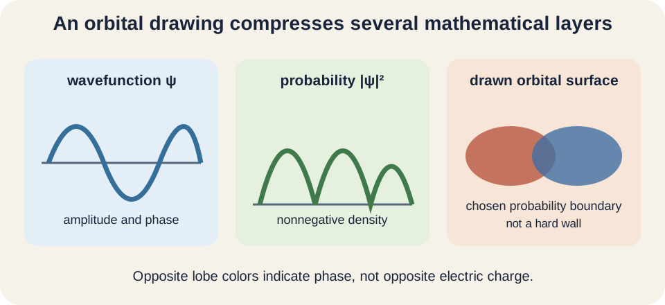
The wavefunction $\psi$ can be positive, negative, or complex, so it is not directly a probability. Probability density is $|\psi|^2=\psi^*\psi$, which is nonnegative. The star indicates complex conjugation. Integrating $|\psi|^2$ over a region gives the probability of detecting the electron there in a position measurement. Normalization makes the probability over all space equal one.

An orbital is a one-electron spatial wavefunction in the atomic model. Textbook boundary surfaces usually enclose a chosen percentage, perhaps ninety percent, of the probability. They are not hard walls. Probability density generally extends beyond the drawn surface. An electron is not a smeared classical bead, but its measurement statistics are distributed.

Principal quantum number organizes shells

The principal quantum number is $n=1,2,3,\ldots$. It labels the principal shell and strongly relates to orbital size and energy. In hydrogen-like atoms, energy depends only on $n$ in the basic nonrelativistic model. Larger $n$ generally corresponds to greater average electron distance and higher energy. In multi-electron atoms, shielding and penetration complicate the ordering.

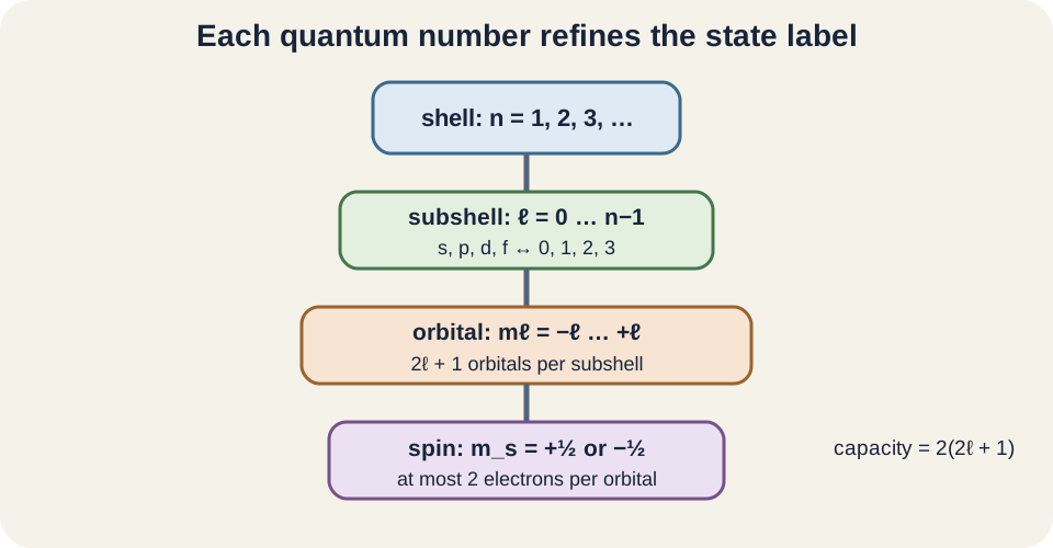
For a given $n$, the angular-momentum quantum number may be $\ell=0,1,\ldots,n-1$. Thus $n=1$ permits only $\ell=0$, while $n=3$ permits $\ell=0,1,2$. The letters $s$, $p$, $d$, and $f$ correspond to $\ell=0,1,2,3$. A label such as $3d$ combines $n=3$ with $\ell=2$. The number and letter carry different information.

The word shell refers to all states sharing $n$. A subshell refers to states sharing both $n$ and $\ell$. Therefore the third shell contains $3s$, $3p$, and $3d$ subshells. A subshell contains one or more orbitals. An orbital can hold zero, one, or two electrons under the Pauli rule.

Magnetic quantum number counts orbitals

For a selected $\ell$, the magnetic quantum number takes integer values $m_\ell=-\ell,-\ell+1,\ldots,0,\ldots,+\ell$. There are $2\ell+1$ allowed values. Each allowed $m_\ell$ labels one orbital within that subshell in the elementary atomic description. An $s$ subshell has one orbital, a $p$ subshell has three, a $d$ subshell has five, and an $f$ subshell has seven. The word “magnetic” reflects angular-momentum behavior in a magnetic field.

For a $p$ subshell, $\ell=1$, so $m_\ell=-1,0,+1$. That gives three orbitals. Familiar real-space drawings are often labeled $p_x$, $p_y$, and $p_z$. These are convenient real linear combinations of angular states rather than literal arrows labeled by $m_\ell$ one-to-one in every treatment. Orientation language is useful but should not be oversimplified.

For a $d$ subshell, $\ell=2$, so $m_\ell=-2,-1,0,+1,+2$. The formula $2\ell+1$ gives five orbitals. At two electrons per orbital, a filled $d$ subshell holds ten electrons. The capacity follows from orbital count and spin, not from memorizing ten independently. This derivation transfers to every subshell.

Spin quantum number and Pauli exclusion

An electron has intrinsic spin angular momentum. In the elementary orbital model, its spin projection quantum number is $m_s=+\frac{1}{2}$ or $m_s=-\frac{1}{2}$. These two values are often drawn as upward and downward arrows. The arrows do not mean the electron is a tiny ball spinning clockwise or counterclockwise. Spin is an intrinsically quantum property.

The Pauli exclusion principle states that no two electrons in one atom can have the same complete set of four quantum numbers. Two electrons can share the same spatial orbital values $n$, $\ell$, and $m_\ell$ only if their $m_s$ values differ. Therefore one orbital holds at most two electrons with opposite spin projections. This rule creates the familiar orbital capacity. It also helps determine electron configurations.

An $s$ subshell has one orbital and capacity two. A $p$ subshell has three orbitals and capacity six. A $d$ subshell has five orbitals and capacity ten. An $f$ subshell has seven orbitals and capacity fourteen. The general subshell capacity is $2(2\ell+1)$ electrons.

Worked example: the 3d subshell

The label $3d$ means $n=3$ and $\ell=2$. For $\ell=2$, allowed $m_\ell$ values are $-2,-1,0,+1,+2$. Therefore the subshell contains five orbitals. Each orbital accepts at most two electrons with opposite spin projections. The maximum capacity is ten electrons.

A valid 3d electron can have a set such as $(n,\ell,m_\ell,m_s)=(3,2,-1,+\frac{1}{2})$. The set $(3,3,0,+\frac{1}{2})$ is invalid because for $n=3$, $\ell$ can only be zero, one, or two. The set $(3,2,3,-\frac{1}{2})$ is invalid because $m_\ell$ must lie from $-2$ to $+2$. Checking ranges in order catches errors. Later quantum numbers depend on earlier ones.

Two electrons in the same 3d orbital share $n$, $\ell$, and $m_\ell$. They must have opposite $m_s$ values. Two electrons with identical four-number sets would violate Pauli exclusion. Electrons in different 3d orbitals may have the same spin projection. Hund’s rule will later describe favorable distribution among degenerate orbitals.

Orbital shape and angular nodes

An $s$ orbital has spherical probability symmetry around the nucleus. A $p$ orbital has two lobes separated by an angular nodal plane in common real drawings. Many $d$ orbitals have four-lobed forms, while one has two lobes plus a toroidal region. These surfaces show selected probability contours and wavefunction phase. They do not depict solid electron material.

The number of angular nodes is $\ell$. Thus an $s$ orbital has zero angular nodes, a $p$ orbital has one, and a $d$ orbital has two. At a node, $\psi=0$ and therefore $|\psi|^2=0$. The electron has zero probability density exactly on the ideal nodal surface. Nodes arise from wave behavior and boundary conditions.

Colors or plus-minus labels on orbital lobes usually represent wavefunction phase, not electric charge. Both lobes of a $p$ orbital describe the same negatively charged electron state. Opposite phase matters when orbitals combine and interfere in bonding. Calling one lobe positive charge is incorrect. A legend should explain every orbital color scheme.

Radial nodes and total node count

For hydrogen-like orbitals, total nodes equal $n-1$. Angular nodes equal $\ell$. Radial nodes therefore equal $n-\ell-1$. A radial node is a spherical radius at which the radial part of the wavefunction crosses zero. Probability density vanishes on that nodal surface.

For a $2s$ orbital, $n=2$ and $\ell=0$. It has zero angular nodes and $2-0-1=1$ radial node. A $2p$ orbital has one angular node and $2-1-1=0$ radial nodes. Both have one total node. Their spatial distributions and penetration differ.

For a $3d$ orbital, $n=3$ and $\ell=2$. It has two angular nodes and zero radial nodes. For $3s$, it has zero angular nodes and two radial nodes. These patterns influence how closely probability penetrates toward the nucleus. In multi-electron atoms, penetration contributes to subshell energy differences.

Hydrogen-like energy and transitions

For a one-electron hydrogen-like species, energy is $E_n=-\frac{13.6\,\mathrm{eV}\,Z^2}{n^2}$. The atomic number $Z$ is nuclear charge magnitude in proton units, $n$ is principal quantum number, and electronvolt is an energy unit. The negative sign indicates a bound state relative to a zero-energy separated electron and nucleus. Larger $n$ gives energy closer to zero. Ionization corresponds to reaching or exceeding the continuum threshold.

For hydrogen, the transition from $n=3$ to $n=2$ has $\Delta E=E_2-E_3$. Since $E_2$ is more negative, the atom’s energy decreases and a photon is emitted. Its magnitude determines frequency by $|\Delta E|=hf$. Transitions ending at a common lower $n$ form a spectral series. The line pattern compresses as higher levels get closer together.

This simple equation does not directly give multi-electron atom energies. Electron–electron repulsion, shielding, penetration, and exchange change the pattern. Spectroscopic terms and computational methods become necessary. The hydrogen result remains a conceptual anchor. Its success and limits both matter.

Multi-electron atoms break simple degeneracy

In ideal hydrogen, orbitals with the same $n$ share energy in the basic model. In multi-electron atoms, energy depends on both $n$ and $\ell$ because electrons shield and repel one another. An $s$ orbital penetrates closer to the nucleus than a $p$ orbital in the same shell. It can experience greater effective nuclear attraction. Subshell energies therefore split.

The common Aufbau ordering is an empirical and theoretical guide for ground-state electron configurations. It is not simply “fill every shell completely before the next.” The $4s$ and $3d$ ordering illustrates the complication, and ion formation can change their relative energies. Exceptions exist because configurations reflect close energy balances. Measured spectra and chemical behavior help establish actual arrangements. A later lesson will handle those occupancy rules carefully.

Orbital diagrams are state-accounting tools. Boxes or lines represent orbitals, while arrows represent electron spin projections. They do not show physical containers or actual arrow-shaped electrons. The diagram suppresses spatial probability information to emphasize occupancy. Every representation selects some features and omits others.

Quantum measurement and uncertainty

Probability in quantum mechanics is not merely ignorance about a hidden ordinary orbit in the basic theory. Repeated position measurements on identically prepared states produce a distribution predicted by $|\psi|^2$. A single measurement yields one localized outcome. Repeating the preparation reconstructs the statistical pattern. The orbital describes the state before the measurement outcome.

Position and momentum cannot both be specified with unlimited precision. Heisenberg’s uncertainty relation is $\Delta x\Delta p_x\geq\frac{\hbar}{2}$. Here $\Delta x$ and $\Delta p_x$ are statistical spreads, and $\hbar=\frac{h}{2\pi}$. The relation is not simply poor instrument craftsmanship. It is a structural feature of quantum states.

This uncertainty undermines a precise planetary trajectory. A classical path requires both position and momentum at each instant. Atomic orbitals instead provide stationary-state probability and phase structure. Classical intuition remains useful for some averages and correspondences. It must not overwrite the quantum claims.

Common misconceptions and repairs

One misconception treats shells as literal circular tracks. A shell collects states with common principal quantum number. Its orbitals can have different shapes and penetration. Probability density extends across ranges rather than one fixed radius. Replace track drawings with state labels and distributions.

Another misconception says an orbital contains a fixed cloud substance. The cloud image represents detection probability density across repeated measurements. A boundary surface is chosen for visualization and is not impermeable. Wavefunction phase may change sign across nodes even though probability remains nonnegative. Legend and wording should preserve these distinctions.

A third misconception confuses orbital count with electron count. A $p$ subshell contains three orbitals and up to six electrons. A $d$ subshell contains five orbitals and up to ten electrons. The factor two comes from allowed opposite spin projections. Derive capacity instead of guessing from the letter.

Practice with guided feedback

First, find photon energy for wavelength $500\,\mathrm{nm}$. Second, list allowed $\ell$ values for $n=4$. Third, determine orbitals and capacity for an $f$ subshell. Fourth, find angular and radial nodes for $3p$. Explain every symbol and convert all units before arithmetic.

For $500\,\mathrm{nm}$, $E=\frac{hc}{\lambda}=3.97\times10^{-19}\,\mathrm J$ per photon. For $n=4$, allowed $\ell$ values are $0,1,2,3$. An $f$ subshell has $\ell=3$, so it contains $2(3)+1=7$ orbitals and holds at most fourteen electrons. A $3p$ orbital has one angular node and $3-1-1=1$ radial node. Its total node count is two.

Check each quantum-number set hierarchically. Principal $n$ must be a positive integer. Then $\ell$ must be below $n$, $m_\ell$ must lie between $-\ell$ and $+\ell$, and $m_s$ must be plus or minus one half. Check photon trends as well: shorter wavelength must give larger energy. These constraints make self-correction possible.

Retrieval and connection forward

Without looking back, explain how line spectra support energy quantization. Write both photon-energy equations and define each symbol with units. Distinguish wavefunction, probability density, orbital, subshell, and shell. Generate all quantum-number values for a $3p$ electron. Derive its orbital count, capacity, and node counts.

Electron-configuration lessons will apply the Aufbau principle, Pauli exclusion, and Hund’s rule. Periodic trends will connect configurations to effective nuclear charge and shielding. Bonding lessons will combine atomic orbitals into molecular descriptions. Spectroscopy will connect transitions with selection rules and instrument observations. Each topic depends on treating orbitals as quantum states rather than classical paths.

Keep one organizing statement: atomic spectra reveal discrete energy differences, and quantum mechanics represents allowed electron states with wavefunctions. Probability density is the squared magnitude of a wavefunction. Quantum numbers organize shells, subshells, orbitals, and spin projections under strict value rules. Nodes and shapes express wave structure. Electron configurations are the next accounting layer built upon this state framework.