Integrals Turn Rates into Accumulation

Suppose a flow meter reports a changing rate in liters per second. One reading describes how quickly water passes at one instant, not how much water has passed over an interval. To recover volume, we must combine many local rate contributions across time. Constant rate permits ordinary multiplication, but changing rate requires increasingly fine approximations. The definite integral is the limit toward which those approximations converge.

Integration is therefore not merely a procedure for finding antiderivatives. Its foundational meaning is accumulation: multiply a local value by a small input width, then add those contributions across an interval. That structure explains area, displacement, mass from density, charge from current, and probability from a probability density. Signs determine whether contributions reinforce or cancel, while units reveal what the final quantity means. The Fundamental Theorem of Calculus connects this global accumulation with the local rate measured by a derivative.

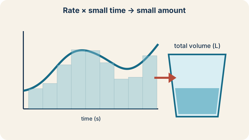
A local rate multiplied by a short duration gives a small amount. Adding many such amounts approximates the total. Narrower time strips allow the rate to vary less within each strip. The definite integral is the limiting total as the widest strip shrinks toward zero. Units change from liters per second times seconds to liters.

Begin with finite accumulation

If velocity remains $6\,\frac{\mathrm{m}}{\mathrm{s}}$ for $4\,\mathrm{s}$, displacement equals rate times duration. The calculation is $(6\,\frac{\mathrm{m}}{\mathrm{s}})(4\,\mathrm{s})=24\,\mathrm{m}$. Seconds cancel between numerator and denominator, leaving metres. This unit cancellation is part of the meaning, not optional decoration. Constant-rate accumulation is multiplication because every equal time slice contributes at the same rate.

Now suppose velocity is $2\,\frac{\mathrm{m}}{\mathrm{s}}$ for $2\,\mathrm{s}$ and then $5\,\frac{\mathrm{m}}{\mathrm{s}}$ for $3\,\mathrm{s}$. The first interval contributes $(2\,\frac{\mathrm{m}}{\mathrm{s}})(2\,\mathrm{s})=4\,\mathrm{m}$. The second contributes $(5\,\frac{\mathrm{m}}{\mathrm{s}})(3\,\mathrm{s})=15\,\mathrm{m}$. Adding gives a total displacement of $19\,\mathrm{m}$. This is integration in finite form because local products are summed across intervals.

The same pattern works beyond motion. A machine producing $12$ parts per hour for $3$ hours produces $36$ parts. A cable with constant linear density $0.8\,\frac{\mathrm{kg}}{\mathrm{m}}$ over $5\,\mathrm{m}$ has mass $4.0\,\mathrm{kg}$. A constant electric current of $2\,\mathrm{A}$ flowing for $10\,\mathrm{s}$ transports $20\,\mathrm{C}$ because $1\,\mathrm{A}=1\,\frac{\mathrm{C}}{\mathrm{s}}$. In every example, a rate or density multiplies an input width to produce an accumulated quantity.

Partition an interval into manageable pieces

Let a function $f$ be defined on the interval $[a,b]$. A partition divides that interval using points $a=x_0<x_1<\cdots<x_n=b$. The symbol $n$ is the number of subintervals, not necessarily the number of distinct physical events. The $i$th subinterval is $[x_{i-1},x_i]$. Its width is $\Delta x_i=x_i-x_{i-1}$, where the Greek capital delta means a finite change.

Choose a sample point $x_i^*$ inside each subinterval. The superscript star identifies the selected representative input and does not mean exponentiation. If $f$ changes little over that subinterval, then $f(x_i^*)$ represents its local value. The approximate contribution is $f(x_i^*)\Delta x_i$. The function value supplies a local height, rate, or density, while the width supplies how much input it acts over.

Adding all contributions produces the Riemann sum $\sum_{i=1}^{n}f(x_i^*)\Delta x_i$. The Greek capital sigma $\sum$ directs us to add one term for every index from $i=1$ through $i=n$. Different sample rules create left-endpoint, right-endpoint, midpoint, or more general sums. Coarse partitions can produce visibly different answers because the function varies inside each piece. The essential question is whether those differences vanish as every subinterval becomes small.

Define the definite integral as a limit

The definite integral is defined by $\int_a^b f(x)\,dx=\lim_{\max \Delta x_i\to0}\sum_{i=1}^{n}f(x_i^*)\Delta x_i$ when the limit exists independently of acceptable sample choices. The elongated symbol $\int$ represents continuous summation. The lower limit $a$ is the starting input, and the upper limit $b$ is the ending input. The expression $dx$ identifies the integration variable and recalls the shrinking widths. The entire expression denotes one accumulated number rather than a new function of $x$.

The condition $\max\Delta x_i\to0$ means that the widest subinterval shrinks toward zero. It is stronger than requiring only the average width to shrink because one coarse piece could otherwise remain. As the mesh becomes fine, a continuous function varies less inside each individual piece. Left, right, and midpoint choices then approach the same total. The limit removes the approximation error without treating any physical width as literally equal to zero.

Not every arbitrary function is integrable under every theory of integration, but continuous functions on closed intervals are Riemann integrable. Functions with finitely many jump discontinuities are also commonly Riemann integrable. Foundational calculus therefore works with a broad and useful class of functions. The definition matters because it explains what calculator and antiderivative methods are calculating. Integration rules are efficient consequences of this limiting accumulation, not replacements for its meaning.

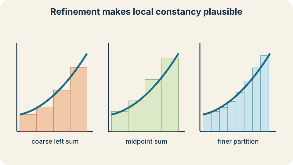
Different sample points produce different coarse rectangle sums. Left endpoints use the function value at the start of each piece. Right endpoints use the value at the end, while midpoint sums use the center. Refinement reduces the width of every rectangle. For an integrable function, all legitimate sufficiently fine choices converge to the same definite integral. The common limit is independent of the sampling rule.

Construct a Riemann sum for a linear function

Divide $[0,1]$ into $n$ equal pieces. Every width is $\Delta x=\frac{1-0}{n}=\frac{1}{n}$. For right endpoints, the sample point in piece $i$ is $x_i^*=\frac{i}{n}$. With $f(x)=x$, the local contribution is $f(x_i^*)\Delta x=\frac{i}{n}\frac{1}{n}$. Adding the contributions gives $R_n=\frac{1}{n^2}\sum_{i=1}^{n}i$.

The finite-sum identity $\sum_{i=1}^{n}i=\frac{n(n+1)}{2}$ simplifies the expression. Substitution gives $R_n=\frac{n(n+1)}{2n^2}=\frac{1}{2}+\frac{1}{2n}$. The first term is the limiting value, while the second is the right-sum error for this example. As $n\to\infty$, the fraction $\frac{1}{2n}$ approaches zero. Therefore $\int_0^1x\,dx=\frac{1}{2}$.

The estimate direction can be predicted before calculating. Because $f(x)=x$ increases, the right endpoint supplies the largest height in every subinterval. Each right rectangle therefore lies above the graph except at its right edge. Right sums overestimate the integral, exactly as the positive error term shows. Left sums underestimate, and both families squeeze toward the same limit.

Interpret sign as orientation

A definite integral measures signed accumulation. Contributions where $f(x)>0$ are positive because positive height multiplies positive width. Contributions where $f(x)<0$ are negative. The integral combines them algebraically, so opposite signs can cancel. This behavior is necessary in applications such as displacement, net flow, and net change.

For $f(x)=x$ on $[-1,1]$, symmetry gives $\int_{-1}^{1}x\,dx=0$. The contribution on $[-1,0]$ is negative, and the equal-magnitude contribution on $[0,1]$ is positive. Zero net accumulation does not mean the graph encloses no geometric region. It means the signed contributions balance. The integral of $|x|$ instead is $\int_{-1}^{1}|x|\,dx=1$ square unit.

Reversing the bounds reverses orientation. The identity $\int_b^a f(x)\,dx=-\int_a^b f(x)\,dx$ follows because traversal proceeds in the opposite direction. Equal bounds produce $\int_a^a f(x)\,dx=0$ because there is no interval width to accumulate. These properties resemble displacement along an oriented route. They also explain why a definite integral is more general than unsigned geometric area.

Use units to identify the accumulated quantity

If $v(t)$ is measured in $\frac{\mathrm{m}}{\mathrm{s}}$ and $dt$ carries seconds, then $v(t)dt$ has metres. Thus $\int_{t_1}^{t_2}v(t)\,dt$ represents displacement in metres. If linear density $\rho(x)$ is measured in $\frac{\mathrm{kg}}{\mathrm{m}}$ and $dx$ carries metres, then $\int_a^b\rho(x)\,dx$ represents mass in kilograms. Unit multiplication exposes the physical meaning before any numerical evaluation. The surviving unit names the accumulated output.

A probability density has units reciprocal to its input. If $p(x)$ describes a continuous length measurement in metres, its units are $\mathrm{m}^{-1}$. The product $p(x)dx$ is dimensionless, as probability must be. Integrating over all possible values gives $1$. Integrating over a subinterval gives the probability assigned to that range, not the probability of one exact continuous value.

Units can also reveal a wrong model. Integrating position measured in metres with respect to seconds produces metre-seconds, not displacement. Differentiating position with respect to time produces velocity, while integrating velocity produces displacement. Before calculating, write the integrand units times the integration-variable units. If the product does not match the intended output, reconsider the quantity being accumulated.

Build an accumulation function

Fix a starting point $a$ and define $A(x)=\int_a^x f(t)\,dt$. The symbol $t$ is a dummy integration variable, while $x$ remains the variable upper endpoint. Changing the letter $t$ inside the integral would not change the value. The function $A$ records how much signed accumulation has occurred from $a$ to each possible endpoint $x$. Unlike a definite integral with two fixed bounds, it produces a function.

If the endpoint increases from $x$ to $x+h$, the added accumulation is $A(x+h)-A(x)=\int_x^{x+h}f(t)\,dt$. For small $h$, the function is nearly $f(x)$ over that short interval. The added amount is therefore approximately $f(x)h$. Dividing by $h$ gives $\frac{A(x+h)-A(x)}{h}\approx f(x)$. Taking the limit as $h\to0$ yields $A'(x)=f(x)$ when $f$ is continuous.

This result is Part I of the Fundamental Theorem of Calculus. In symbols, $\frac{d}{dx}\int_a^x f(t)\,dt=f(x)$. Differentiation asks for the local rate at which accumulation changes. Adding a thin interval at the upper endpoint contributes at the current height $f(x)$. Accumulating a continuous rate and then differentiating therefore recovers the original rate.

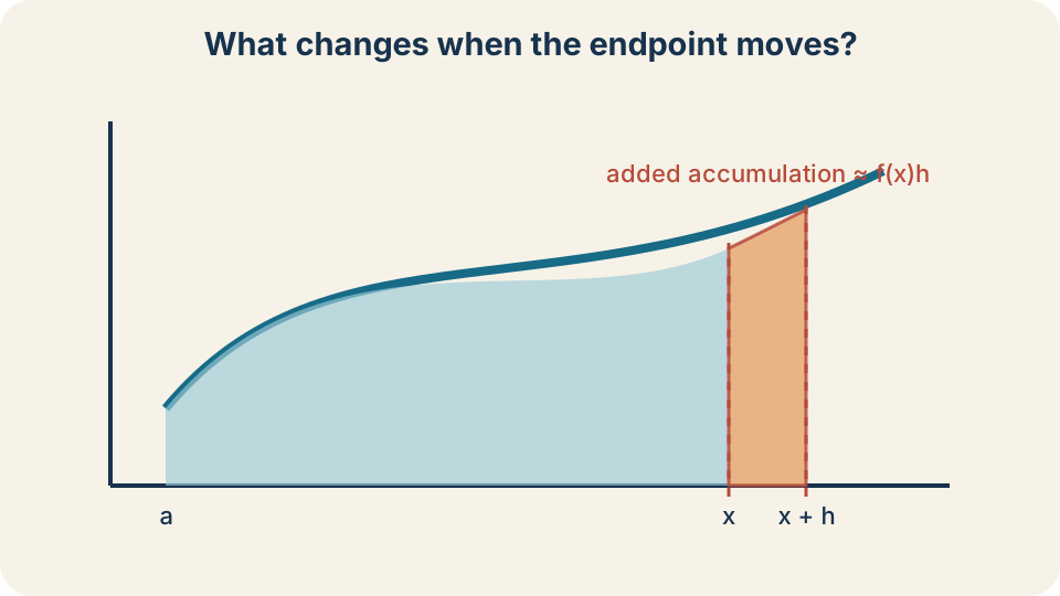
Moving the upper endpoint from $x$ to $x+h$ adds one thin region. Its width is $h$, and its height is approximately $f(x)$. The added accumulation is therefore approximately $f(x)h$. Dividing by $h$ estimates the accumulation function’s derivative. The limit makes the estimate exact for continuous $f$. This local strip explains the first part of the Fundamental Theorem.

Evaluate with an antiderivative

Part II of the Fundamental Theorem states that if $F'(x)=f(x)$ on $[a,b]$, then $\int_a^b f(x)\,dx=F(b)-F(a)$. The function $F$ is an antiderivative of $f$. Evaluating at the upper endpoint and subtracting the lower endpoint replaces the limiting sum with an efficient calculation. The theorem does not redefine the integral as endpoint subtraction. It proves that endpoint subtraction equals the accumulated limit under the stated conditions.

For example, an antiderivative of $f(x)=3x^2$ is $F(x)=x^3$. Therefore $\int_1^4 3x^2\,dx=4^3-1^3=63$. If $x$ is measured in metres and $f$ is a density in $\frac{\mathrm{kg}}{\mathrm{m}}$, the numerical result would carry kilograms after the model’s scale factors were included. The endpoint calculation is fast, but the sign and units still come from accumulation. Always interpret the result in the context that produced the integrand.

The indefinite notation $\int f(x)\,dx=F(x)+C$ denotes a family of antiderivatives. The constant $C$ is required because differentiation erases constants. A definite integral is a number when both bounds are fixed, while an indefinite integral represents functions. In $F(b)-F(a)$, the same constant cancels. Confusing these two uses of the integral symbol obscures whether the requested output is a number or a family.

Separate displacement from total distance

Let velocity be $v(t)=3t^2-6t$ in $\frac{\mathrm{m}}{\mathrm{s}}$ on $0\,\mathrm{s}\le t\le3\,\mathrm{s}$. An antiderivative is $V(t)=t^3-3t^2$ with units of metres. Displacement is $\int_0^3v(t)\,dt=V(3)-V(0)=0\,\mathrm{m}$. The zero means the final position equals the initial position. It does not mean the object remained still.

Total distance counts motion in either direction positively. Factor velocity as $v(t)=3t(t-2)$ to locate zeros at $t=0\,\mathrm{s}$ and $t=2\,\mathrm{s}$. Velocity is negative on $(0,2)$ and positive on $(2,3)$. Distance is therefore $-\int_0^2v(t)\,dt+\int_2^3v(t)\,dt$. Evaluating gives $4\,\mathrm{m}+4\,\mathrm{m}=8\,\mathrm{m}$.

The sign split is a conceptual step rather than mere algebra. Integrating velocity directly yields net displacement because backward and forward motions cancel. Integrating $|v(t)|$ yields total distance because every contribution becomes nonnegative. A graph of velocity helps identify sign-change times before calculation. The same distinction appears between net flow and total throughput or between net profit and total transaction volume.

Approximation remains useful

Many functions lack elementary antiderivatives, and many data sets are known only at sampled points. The definite integral still exists even when symbolic evaluation is unavailable. Numerical rules approximate it using structured weighted sums. Left and right sums are simple, midpoint sums often improve accuracy, and trapezoidal sums connect adjacent data values with line segments. Each method remains an accumulation of local contributions.

Error reasoning should accompany the estimate. For an increasing function, left sums underestimate and right sums overestimate. For a concave-up function, trapezoids generally lie above the graph, while midpoint rectangles often lie below. Comparing refinements can show whether values are stabilizing. An approximation without an estimate of reliability is less informative than one paired with direction or magnitude of error.

Suppose flow readings in $\frac{\mathrm{L}}{\mathrm{s}}$ are available every $0.5\,\mathrm{s}$. Multiplying each representative reading by $0.5\,\mathrm{s}$ gives an estimated number of liters for that interval. Summing produces estimated total volume. Halving the sampling interval usually captures more variation and improves the approximation. The Riemann definition explains why this data-based procedure is mathematically legitimate.

Repair common misconceptions

“Area under the curve” is incomplete language because a definite integral is signed. Regions below the horizontal axis contribute negatively. To calculate geometric area, split at sign changes or integrate an absolute value. The horizontal axis also need not represent physical distance. A graph of rate against time uses rectangle area as a visual proxy for rate-times-time accumulation.

The differential $dx$ should not be discarded as meaningless decoration. It identifies the input variable being accumulated and carries its conceptual units. In multivariable settings, changing the differential changes the geometric measure, such as length, area, or volume. Even in one variable, it distinguishes $\int v(t)\,dt$ from an expression integrated with respect to another variable. Reading the differential aloud as “with respect to $x$” reinforces its role.

An antiderivative is not the same object as a definite integral. The former is a family of functions, while the latter is a signed accumulated number over specified bounds. The Fundamental Theorem connects them but does not erase their distinction. Riemann sums explain what the integral means, and antiderivatives explain how many integrals can be evaluated efficiently. Keeping meaning and method separate makes unfamiliar applications easier to model.

Retrieve the central ideas

If $f$ is negative throughout $[a,b]$ with $a<b$, then $\int_a^b f(x)\,dx$ is negative. Every width is positive, while every sampled function value is negative. Their products are therefore negative, and so are their sums. The limiting accumulation preserves that sign. No graph sketch is required once the signed-product reasoning is clear.

If a flow rate is measured in $\frac{\mathrm{gal}}{\mathrm{min}}$ and integrated with respect to minutes, the output unit is gallons. Minutes cancel in the product $\frac{\mathrm{gal}}{\mathrm{min}}\cdot\mathrm{min}$. If the integral is zero, the rate need not be zero at every instant. Positive and negative flow contributions may cancel. Context determines whether negative flow represents reversal, outflow, or a chosen orientation.

The definite integral is the limit of finite accumulated contributions. A Riemann sum multiplies a representative local value by an input width and adds across the interval. Signs identify orientation or net change, while units identify the accumulated quantity. The Fundamental Theorem states that accumulation functions differentiate back to their rates and that antiderivatives evaluate definite integrals by endpoint change. These ideas together turn local information into a global total.