Velocity Is Change with Direction

Position tells where an object is relative to a chosen origin. Velocity tells how rapidly that position changes and in which coordinate direction. The distinction among position, displacement, distance, velocity, and speed is foundational because each answers a different question. Graphs translate those quantities into slopes, heights, and signed areas. This article builds velocity from measurable intervals and then passes carefully to instantaneous motion.

Define a coordinate system before describing motion

One-dimensional motion requires an origin and a positive direction. A coordinate $x=0\,\mathrm{m}$ marks the origin, while positive and negative values locate positions on opposite sides. Choosing right as positive is common but not mandatory. Choosing left as positive would also work if used consistently. Physical motion does not change when coordinate labels change.

Position is a coordinate, not a traveled amount. An object at $x=-3.0\,\mathrm{m}$ is three meters on the negative side of the origin. The negative sign indicates location relative to the chosen axis. It does not mean the object has a negative size or has traveled a negative distance. Coordinate signs encode direction.

Time also needs a reference. The symbol $t=0\,\mathrm{s}$ marks the chosen start of the clock, not necessarily the beginning of all physical motion. A position function $x(t)$ assigns a coordinate to each time in its domain. The parentheses indicate that position depends on time. Units must accompany both input and output when the function models physical data.

Separate distance from displacement

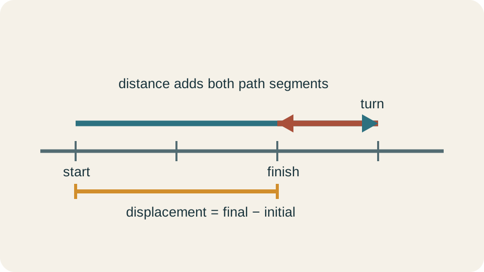
Displacement is the change in position between two events. From time $t_1$ to time $t_2$, it is $\Delta x=x(t_2)-x(t_1)$. The Greek capital delta, $\Delta$, means final value minus initial value. Displacement has units of length. Its sign indicates the net coordinate direction.

Distance traveled is the total path length accumulated during the interval. It is nonnegative and does not cancel when direction reverses. A runner who completes one $400\,\mathrm{m}$ lap returns to the starting position. The displacement is $0\,\mathrm{m}$ while the distance is $400\,\mathrm{m}$. Equal endpoints do not imply that no motion occurred.

In one-direction motion, distance magnitude equals displacement magnitude. After a reversal, they usually differ. Distance depends on the entire path, while displacement depends only on endpoints. This distinction later separates average speed from average velocity. A sketch of the coordinate line can expose which quantity a problem is requesting.

Calculate average velocity

Average velocity over an interval is $v_{\mathrm{avg}}=\dfrac{\Delta x}{\Delta t}$. The time change is $\Delta t=t_2-t_1$. The numerator is displacement rather than distance traveled. Average velocity therefore describes net position change per elapsed time. Its direction follows the sign of $\Delta x$ when $\Delta t$ is positive.

Suppose an object moves from $x_1=2.0\,\mathrm{m}$ at $t_1=1.0\,\mathrm{s}$ to $x_2=14.0\,\mathrm{m}$ at $t_2=5.0\,\mathrm{s}$. The displacement is $14.0\,\mathrm{m}-2.0\,\mathrm{m}=12.0\,\mathrm{m}$. The elapsed time is $5.0\,\mathrm{s}-1.0\,\mathrm{s}=4.0\,\mathrm{s}$. Therefore $v_{\mathrm{avg}}=\dfrac{12.0\,\mathrm{m}}{4.0\,\mathrm{s}}=3.0\,\mathrm{\dfrac{m}{s}}$. The positive sign indicates net motion in the positive direction.

Average velocity ignores detailed motion between endpoints. The object could stop, reverse briefly, or change speed while preserving the same endpoint data. Many position histories can share one average velocity. The measure summarizes an interval rather than reconstructing its path. Additional observations are needed to describe what happened inside.

Distinguish average speed

Average speed is total distance traveled divided by elapsed time. It is a nonnegative scalar quantity. Average velocity uses signed displacement instead. If motion never reverses in one dimension, average speed equals the magnitude of average velocity. If motion reverses, average speed is larger unless net displacement still equals total distance magnitude.

Suppose a cyclist travels $60.0\,\mathrm{m}$ east and then $20.0\,\mathrm{m}$ west in $20.0\,\mathrm{s}$. Taking east as positive, displacement is $+40.0\,\mathrm{m}$. Average velocity is $+2.00\,\mathrm{\dfrac{m}{s}}$. Distance is $80.0\,\mathrm{m}$, so average speed is $4.00\,\mathrm{\dfrac{m}{s}}$. The two values answer different questions.

The word “speed” should not be used casually for a signed value. A vehicle’s speedometer reports magnitude, not coordinate direction. Navigation systems use velocity because direction matters. Collision and momentum calculations also require vector direction. Clear vocabulary prevents lost signs from becoming physical errors.

Read average velocity as secant slope

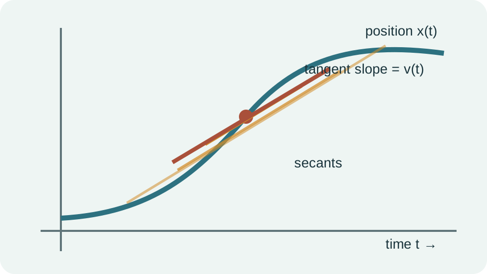
On a position-versus-time graph, the points $(t_1,x(t_1))$ and $(t_2,x(t_2))$ define a secant line. Its slope is $\dfrac{x(t_2)-x(t_1)}{t_2-t_1}$. This is exactly the average-velocity formula. Horizontal change represents elapsed time. Vertical change represents displacement.

A steep positive secant has a large positive average velocity. A steep negative secant has a large negative average velocity. A horizontal secant has zero average velocity even if the graph wandered between endpoints. Slope combines magnitude and direction in one signed number. Axis units determine slope units.

Graph scale matters visually. Stretching the horizontal axis can make the same physical slope appear flatter. Numerical slope must be calculated from labeled coordinate changes rather than judged only by appearance. Units such as meters per second provide an invariant interpretation. A graph communicates motion only when axes and scales are read.

Approach instantaneous velocity through a limit

Average velocity describes an interval, but motion may change during that interval. To describe velocity at time $t$, compare position at $t$ with position at nearby time $t+\Delta t$. The interval estimate is $\dfrac{x(t+\Delta t)-x(t)}{\Delta t}$. Smaller nonzero values of $\Delta t$ focus more locally. The numerator and denominator both approach zero, but their ratio may approach a finite value.

Instantaneous velocity is $v(t)=\lim_{\Delta t\to0}\dfrac{x(t+\Delta t)-x(t)}{\Delta t}$. The arrow means that the time interval approaches zero without being set equal to zero. Directly substituting zero would create the undefined quotient $0/0$. The limit asks what the secant slopes approach. That limiting slope is the tangent slope at time $t$.

Derivative notation compresses this definition to $v(t)=\dfrac{dx}{dt}=x'(t)$. The expression $dx/dt$ names the derivative of position with respect to time. It is not an ordinary fraction, although its unit behavior resembles one. The prime in $x'(t)$ is another derivative notation. All three forms describe instantaneous rate of positional change.

Derive velocity from a position formula

Let position be $x(t)=\left(3.00\,\mathrm{\dfrac{m}{s^2}}\right)t^2$. The coefficient has units of meters per square second. Multiplying by $t^2$ produces meters, as a position formula requires. Applying the power rule gives $v(t)=\left(6.00\,\mathrm{\dfrac{m}{s^2}}\right)t$. Differentiation lowers the time power from two to one and multiplies by two.

At $t=2.00\,\mathrm{s}$, velocity is $v=(6.00\,\mathrm{\dfrac{m}{s^2}})(2.00\,\mathrm{s})=12.0\,\mathrm{\dfrac{m}{s}}$. One factor of seconds cancels from the denominator. The positive result indicates motion in the positive coordinate direction. The value increases with time because the position curve becomes steeper. Units and graph shape agree with the derivative.

At $t=0\,\mathrm{s}$, velocity is zero even though the coefficient in the position function is not zero. The position graph has a horizontal tangent there. After that instant, the positive slope grows. An object can be momentarily at rest while its velocity is changing. Instantaneous rest does not imply permanent rest.

Interpret motion from a position graph

The height of a position graph gives position, not velocity. Velocity is represented by slope. A graph above the time axis can still have negative velocity if it slopes downward. A graph below the axis can have positive velocity if it slopes upward. Position sign and velocity sign describe different features.

A horizontal segment means constant position and therefore zero velocity. A straight sloped segment means constant velocity. A curved segment means slope changes and therefore velocity changes. A local maximum or minimum has horizontal tangent when the function is differentiable. Such a point is a candidate for reversal because velocity is zero.

Zero velocity alone does not guarantee reversal. The function $x(t)=t^3$ has zero derivative at $t=0$ but continues increasing through that time. Its slope is positive on both sides except at the instant itself. A reversal requires velocity to change sign. Inspecting intervals on both sides distinguishes a stop-and-reverse from a momentary flattening.

Interpret motion from a velocity graph

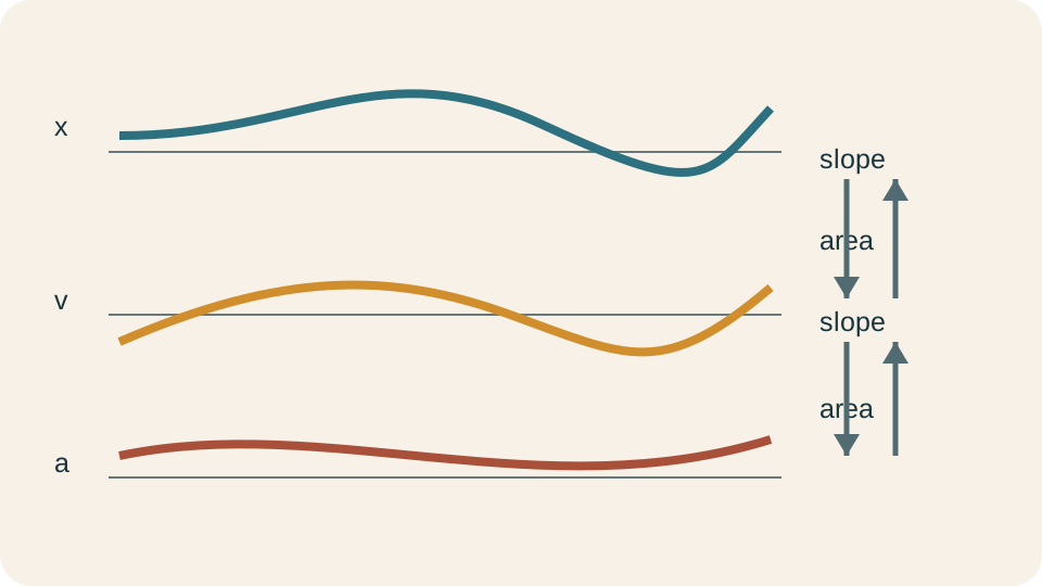
On a velocity-versus-time graph, height directly gives instantaneous velocity. Values above zero represent positive-direction motion. Values below zero represent negative-direction motion. Crossings of zero mark candidate reversals. The graph’s slope represents acceleration rather than velocity.

Signed area under the velocity graph gives displacement. From time $a$ to time $b$, $x(b)-x(a)=\int_a^b v(t)\,dt$. The integral sign represents continuous accumulation. Area above the time axis contributes positive displacement. Area below contributes negative displacement.

Total distance requires accumulating speed, which is $|v(t)|$. Therefore distance traveled is $\int_a^b|v(t)|\,dt$. Absolute-value bars make negative velocities contribute positive path length. Splitting the interval at velocity zeros often simplifies calculation. Displacement and distance agree only when velocity does not change sign.

Relate velocity and acceleration signs

Acceleration is the time derivative of velocity, written $a(t)=\dfrac{dv}{dt}$. It is also the second time derivative of position, $a(t)=\dfrac{d^2x}{dt^2}$. Acceleration units are length per square time, such as meters per square second. Its sign describes the direction of velocity change. It does not by itself say whether the object is speeding up.

An object speeds up when velocity and acceleration share the same sign. Positive velocity with positive acceleration increases positive speed magnitude. Negative velocity with negative acceleration makes velocity more negative, also increasing magnitude. An object slows down when velocity and acceleration have opposite signs. Direction and change of speed must be analyzed separately.

For $x(t)=t^3-3t$ in compatible units, $v(t)=3t^2-3$ and $a(t)=6t$. On $0<t<1$, velocity is negative while acceleration is positive. The object moves in the negative direction but slows because velocity approaches zero. At $t=1$, velocity changes from negative to positive and the object reverses. After the reversal, positive velocity and positive acceleration make its speed increase.

Estimate velocity from discrete measurements

Experimental position data arrive at separate times rather than as a perfect formula. A forward difference estimates velocity at $t_i$ by $\dfrac{x_{i+1}-x_i}{t_{i+1}-t_i}$. This average velocity belongs naturally to the interval between the measurements. Assigning it exactly to the left endpoint is an approximation. Smaller intervals usually improve local resolution when noise is modest.

A central difference estimates velocity at an interior time using measurements on both sides. For equally spaced times, $v(t_i)\approx\dfrac{x(t_i+h)-x(t_i-h)}{2h}$. The symbol $h$ is the time spacing. Symmetry often cancels part of the approximation error. Endpoint estimates require different formulas because data do not exist on both sides.

Differentiation amplifies measurement noise. Subtracting two nearly equal noisy positions can make error large relative to the small displacement. Reducing time spacing too far may worsen the velocity estimate even though the mathematical approximation improves. Smoothing or model-based estimation can help, but it introduces assumptions. Sampling rate and measurement precision must be balanced.

Work with vector velocity

In more than one dimension, position is a vector $\mathbf r(t)$. Boldface distinguishes a vector from the scalar residual notation used in other contexts. Velocity is $\mathbf v(t)=\dfrac{d\mathbf r}{dt}$. Each coordinate is differentiated with respect to time. The velocity vector is tangent to the trajectory.

If $\mathbf r(t)=x(t)\widehat{\mathbf i}+y(t)\widehat{\mathbf j}$, then $\mathbf v(t)=\dfrac{dx}{dt}\widehat{\mathbf i}+\dfrac{dy}{dt}\widehat{\mathbf j}$. The unit vectors $\widehat{\mathbf i}$ and $\widehat{\mathbf j}$ mark horizontal and vertical directions. Speed is the magnitude $|\mathbf v|=\sqrt{v_x^2+v_y^2}$. It is nonnegative even when components are negative. The square-root expression follows from the Pythagorean theorem applied to perpendicular velocity components.

A circular trajectory can have constant speed while velocity changes continuously. The tangent direction rotates even if magnitude stays fixed. This change in velocity requires acceleration toward the center. One-dimensional intuition that velocity change means speed change is therefore incomplete. Vectors separate directional change from magnitude change.

Preserve units and significant figures

Every numerical motion quantity should carry units. Writing $9.8$ without context does not identify acceleration, velocity, or another quantity. Gravitational acceleration near Earth’s surface is approximately $9.81\,\mathrm{\dfrac{m}{s^2}}$. A velocity might be $9.81\,\mathrm{\dfrac{m}{s}}$. Fractional unit form makes the distinction visible.

Derivative units follow output units divided by input units. If $x$ is measured in kilometers and $t$ in hours, velocity is measured in kilometers per hour. A second derivative has kilometers per square hour. Converting units midway requires applying conversion factors to the complete quantity. Dimensional consistency is an algebraic check before numbers are trusted.

Significant figures should reflect input precision and model assumptions. Reporting $3.14159265\,\mathrm{\dfrac{m}{s}}$ from positions measured to the nearest tenth of a meter implies false precision. Keep guard digits during intermediate calculations. Round the final result appropriately and state approximation with $\approx$. Numerical detail is not the same as measurement certainty.

Connect velocity to navigation measurements

Satellite navigation estimates position at successive times and can infer velocity from changing coordinates. Doppler shifts in received signals can also provide velocity-related information. Position estimates may be noisy or temporarily unavailable. Finite differences then amplify that noise. Filtering combines multiple measurements and a motion model.

An accelerometer measures specific force related to changes in velocity, not absolute position. Integrating acceleration estimates velocity, and integrating again estimates position. Small sensor bias accumulates over time during integration. Satellite measurements can correct long-term drift. Combining complementary sensors produces better navigation than either source alone.

The mathematical links remain derivatives and integrals. Position differentiation yields velocity, while velocity integration yields displacement. Real systems add sampling, noise, coordinate transformations, and uncertainty. The foundational formulas still organize the computation. Engineering reliability comes from acknowledging the gap between ideal functions and measured data.

Diagnose common motion errors

Negative velocity does not mean slowing down. It means motion in the negative coordinate direction. Whether speed decreases depends on acceleration’s sign relative to velocity. Negative position also does not imply negative velocity. Each sign must be interpreted according to its own quantity.

Another error is using distance in the average-velocity numerator. Average velocity uses displacement. Average speed uses distance. A round trip can therefore have zero average velocity and nonzero average speed. Writing definitions before substitution prevents the quantities from being interchanged.

A third error is reading graph height when slope is required. Position-graph height gives location, while its slope gives velocity. Velocity-graph height gives velocity, while its area gives displacement. Labeling axes and units before interpreting a feature prevents category mistakes. Every graph question should begin by naming what each axis represents.

Practice a complete motion analysis

Suppose $x(t)=(2.00\,\mathrm{m})+(4.00\,\mathrm{\dfrac{m}{s}})t-(1.50\,\mathrm{\dfrac{m}{s^2}})t^2$. The constant term is initial position. The linear coefficient contributes initial velocity. Differentiation gives $v(t)=4.00\,\mathrm{\dfrac{m}{s}}-(3.00\,\mathrm{\dfrac{m}{s^2}})t$. A second derivative gives $a(t)=-3.00\,\mathrm{\dfrac{m}{s^2}}$.

The object stops when $v=0$. Solving $0=4.00\,\mathrm{\dfrac{m}{s}}-(3.00\,\mathrm{\dfrac{m}{s^2}})t$ gives $t=1.33\,\mathrm{s}$. Before this time, velocity is positive. After this time, velocity is negative. The sign change confirms a reversal.

Its position at the reversal is approximately $x(1.33\,\mathrm{s})=4.67\,\mathrm{m}$. Units are produced consistently by every term in the position expression. The downward-opening position curve has a local maximum there. Its tangent is horizontal because velocity is zero. Formula, graph, and sign analysis tell the same story.

Consolidate velocity reasoning

Position is a coordinate relative to an origin. Displacement is endpoint position change, while distance is accumulated path length. Average velocity is displacement divided by elapsed time. Instantaneous velocity is the limiting local rate of positional change. Speed is velocity magnitude.

On a position graph, velocity is slope. On a velocity graph, velocity is height and displacement is signed area. Acceleration is velocity’s slope. Signs reveal coordinate direction and whether speed grows only when velocity and acceleration are considered together. These translation rules connect algebra, calculus, graphs, and physical motion.

A strong solution declares coordinates, writes units, selects the correct definition, and checks graph behavior. It distinguishes interval averages from instantaneous values. It also recognizes measurement noise when derivatives are estimated from data. Velocity is not merely a number attached to motion. It is a directional rate whose meaning depends on reference frame, time, and representation.