Temperature and Thermal Equilibrium

Temperature is a state variable that predicts the direction of spontaneous energy transfer by heating. It is not the amount of energy stored in an object, nor is it identical to the average speed of every particle. We measure temperature by allowing a thermometer and a system to approach thermal equilibrium, then reading a calibrated thermometric property. The zeroth law makes that comparison logically consistent across different systems and instruments. This lesson builds the macroscopic definition first and then connects it cautiously to microscopic models, temperature scales, calorimetry, phase behavior, and measurement limits.

Distinguish temperature from thermal sensation

Human touch is a poor thermometer. A metal object and a wooden object left in the same room can be at the same temperature while the metal feels colder. Metal usually conducts energy away from a warm hand more rapidly, producing a stronger cooling sensation. The skin responds to transfer rate as well as temperature. Thermal sensation therefore depends on material properties, contact, and physiology.

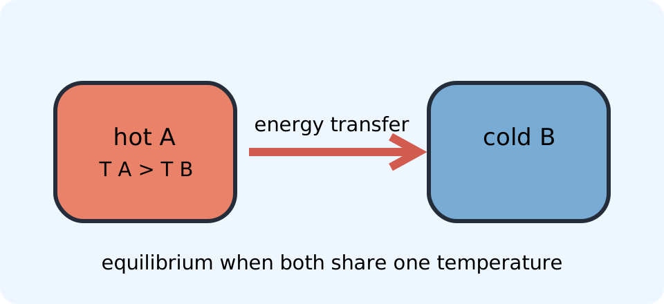
Temperature is an objective state variable measured through a defined procedure. It assigns comparable numerical values to systems and helps predict transfer direction when systems are placed in thermal contact. If system A is hotter than system B, energy tends to transfer from A to B by heating under ordinary conditions. The transfer continues until equilibrium or until another process intervenes. The words hotter and colder refer to temperature ordering rather than stored-energy amount.

A small spark can have very high temperature but little total energy because it contains little matter. A swimming pool can have lower temperature yet vastly greater internal energy. Temperature is intensive, whereas internal energy is extensive. Conflating them makes size and material disappear from the analysis. The distinction becomes especially important in calorimetry and phase change.

Define thermal contact and equilibrium

Two systems are in thermal contact when their boundary permits energy transfer driven by a temperature difference. Direct physical touching is not required because radiation can transfer energy across empty space. A conducting wall permits relatively rapid transfer, while an insulating wall suppresses it under an ideal model. The boundary description determines whether equilibrium can be approached. State which interactions are allowed.

Thermal equilibrium means that macroscopic thermal state variables remain steady and there is no net energy transfer by heating between the systems. Microscopic interactions continue, but transfers in opposite directions balance statistically. Equilibrium is not the same as complete microscopic stillness. It is a macroscopic condition of no net change. Fluctuations remain possible, especially in small systems.

Equilibrium also requires time. A thermometer inserted into a liquid initially has its own temperature and exchanges energy with the liquid. Its reading becomes meaningful only after the relevant thermometric property stabilizes sufficiently. A useful thermometer has small enough thermal capacity that it perturbs the measured system negligibly. Measurement is an interaction, not a passive look at a preexisting number.

Use the zeroth law

The zeroth law states that if system A is in thermal equilibrium with system C and system B is also in thermal equilibrium with system C, then A and B are in thermal equilibrium with each other. The statement gives thermal equilibrium a transitive structure. System C can serve as a thermometer or comparison standard. Direct contact between A and B is unnecessary. This principle makes reproducible temperature measurement possible.

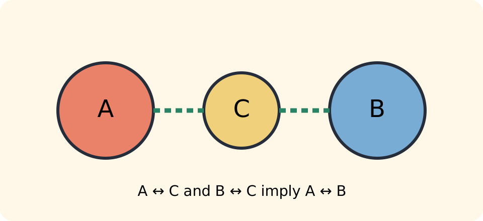
Suppose a calibrated thermometer C reaches the same stable reading when placed separately in contact with A and with B. The zeroth law permits us to assign A and B the same temperature. If A and B were later placed in thermal contact under unchanged conditions, no net heating transfer would occur between them. The thermometer creates a common comparison procedure. Temperature is the numerical property that orders these equilibrium classes.

The name zeroth law arose historically after the first and second laws had already been named. Its conceptual priority justified placing it before the first law in the logical sequence. It does not calculate heat capacity or transfer rate. Instead, it establishes the empirical foundation for saying that temperature is shared at equilibrium. More detailed laws then describe what happens away from equilibrium.

Understand thermometric properties

A thermometric property is a measurable quantity that changes predictably with temperature. Liquid volume, gas pressure at fixed volume, electrical resistance, thermoelectric voltage, emitted spectrum, and semiconductor response can all serve this role. The property must be calibrated against defined reference conditions. A scale converts the measured response into a temperature reading. Different instruments rely on different physical mechanisms.

An ideal linear liquid thermometer might use $X(T)=aT+b$, where $X$ is liquid-column length and $a$ and $b$ are calibration constants. Two reference points can determine the two constants. Real response may be nonlinear, requiring a calibration curve or higher-order model. Interpolation is most reliable within the calibrated range. Extrapolation beyond that range can fail because the material changes phase or response law.

Thermometers also have resolution, accuracy, response time, drift, and uncertainty. Resolution is the smallest displayed increment, while accuracy concerns closeness to a traceable reference. A reading of $25.0\,^{\circ}\mathrm{C}$ does not imply exact knowledge of the true temperature. The uncertainty should reflect calibration and measurement conditions. More displayed digits do not automatically provide more information.

Compare Celsius and Kelvin scales

Kelvin and Celsius intervals have the same size. Their numerical coordinates are related by $T_{\mathrm{K}}=T_{^{\circ}\mathrm{C}}+273.15$. The kelvin value uses the symbol $\mathrm{K}$ without a degree sign. A Celsius temperature uses $^{\circ}\mathrm{C}$. The offset aligns $0\,\mathrm{K}$ with absolute zero.

A sample at $25.0\,^{\circ}\mathrm{C}$ has $T=25.0+273.15=298.15\,\mathrm{K}$. Appropriate rounding depends on the original measurement uncertainty. A change of $10.0\,^{\circ}\mathrm{C}$ equals a change of $10.0\,\mathrm{K}$ because the scale increments match. Absolute coordinates differ by the fixed offset. Difference conversion and coordinate conversion are therefore not the same operation.

Temperature ratios must use an absolute thermodynamic scale. A temperature of $40\,^{\circ}\mathrm{C}$ is not twice $20\,^{\circ}\mathrm{C}$ in an absolute sense because the Celsius origin is offset arbitrarily. Their kelvin values are about $313\,\mathrm{K}$ and $293\,\mathrm{K}$. The ratio is about $1.07$, not $2$. Multiplicative statements require kelvins.

Include the Fahrenheit scale carefully

The Fahrenheit and Celsius coordinates satisfy $T_{^{\circ}\mathrm{F}}=\dfrac95T_{^{\circ}\mathrm{C}}+32$. The slope $\dfrac95$ converts interval sizes, while the intercept $32$ accounts for the different zero. Solving for Celsius gives $T_{^{\circ}\mathrm{C}}=\dfrac59(T_{^{\circ}\mathrm{F}}-32)$. Parentheses matter because the offset must be removed before rescaling. These equations convert coordinates, not thermal energy.

For $68.0\,^{\circ}\mathrm{F}$, Celsius temperature is $\dfrac59(68.0-32)=20.0\,^{\circ}\mathrm{C}$. The corresponding Kelvin temperature is $293.15\,\mathrm{K}$. A Fahrenheit interval of $18.0\,^{\circ}\mathrm{F}$ equals a Celsius or Kelvin interval of $10.0$ degrees. Interval conversion contains no additive offset. Always identify whether the problem gives a reading or a change.

Rankine is an absolute scale with Fahrenheit-sized intervals, although it is less common in introductory science. Its existence reinforces that an interval size and a zero point are separate scale choices. Kelvin is the SI thermodynamic temperature unit. When equations contain ratios, ideal-gas temperature, or powers of absolute temperature, convert to kelvins unless the formula explicitly defines another scale. Unit convention is part of the mathematical model.

Explain why temperature is intensive

An intensive property does not scale directly with system size. Combining two identical samples at $300\,\mathrm{K}$ produces a larger system that remains at $300\,\mathrm{K}$ when no other change occurs. Mass and internal energy approximately double, but temperature does not. Density and pressure are other common intensive properties under suitable conditions. Volume and amount of substance are extensive.

Imagine dividing a uniform equilibrium sample into two equal parts without changing their states. Each half has half the mass and approximately half the internal energy, but both halves have the original temperature. Recombining them reverses the operation. This thought experiment distinguishes state intensity from total amount. Temperature characterizes the thermal state per the equilibrium relation rather than adding across pieces.

Intensive quantities cannot generally be averaged without weights when systems equilibrate. The final temperature depends on masses, heat capacities, phase changes, and energy losses. A simple arithmetic midpoint works only under special symmetry. The equality of initial sample sizes and material properties must be established. “Temperature is intensive” does not mean every mixture temperature is a simple average.

Calculate equilibrium by energy conservation

In an insulated two-body model with no phase change or work, energy lost by the hotter body equals energy gained by the colder body. A constant-specific-heat balance is $m_1c_1(T_f-T_{1i})+m_2c_2(T_f-T_{2i})=0$. The symbol $m$ is mass, $c$ is specific heat capacity, and $T_f$ is their common final equilibrium temperature. Each term has units of joules. Signs emerge from final minus initial temperature.

For equal masses of the same material initially at $20.0\,^{\circ}\mathrm{C}$ and $80.0\,^{\circ}\mathrm{C}$, equal $mc$ factors cancel. The equation becomes $(T_f-20.0\,^{\circ}\mathrm{C})+(T_f-80.0\,^{\circ}\mathrm{C})=0$. Solving gives $T_f=50.0\,^{\circ}\mathrm{C}$. The midpoint follows from equal thermal capacities. It is not a universal equilibrium rule.

Suppose instead that the cold sample has twice the product $mc$ of the hot sample. The final temperature lies closer to the cold initial temperature because more energy is required to change that sample by each degree. The result must lie between initial temperatures for the simple isolated, no-phase-change model. A value outside that interval signals an algebra, sign, or omitted-energy error. Bounds provide a physical check.

Connect temperature to microscopic distributions

For a monatomic ideal gas at equilibrium, mean translational kinetic energy per particle is $\langle K_{\mathrm{trans}}\rangle=\dfrac32k_BT$. The angle brackets denote an ensemble average, $k_B=1.381\times10^{-23}\,\mathrm{\dfrac{J}{K}}$ is Boltzmann’s constant, and $T$ is absolute temperature. The relation connects a macroscopic state variable with a statistical microscopic average. It does not say every molecule has the same kinetic energy. Molecular energies form a distribution.

At higher temperature, the speed distribution shifts and broadens. Some particles move more slowly than the average and others much faster. Collisions continuously redistribute energy while maintaining an equilibrium distribution. Temperature characterizes the distribution, not one representative particle trajectory. This statistical view explains why microscopic fluctuations coexist with stable macroscopic readings.

The phrase “temperature is average kinetic energy” is too broad. In solids, vibrational motion and interatomic potential energy contribute to internal energy. Polyatomic molecules can rotate and vibrate, and interacting fluids have potential-energy structure. Systems with quantum restrictions may activate degrees of freedom only over certain temperature ranges. The ideal monatomic relation is a model-specific bridge rather than a universal definition.

Interpret absolute zero

Absolute zero is $0\,\mathrm{K}=-273.15\,^{\circ}\mathrm{C}$. It is the lower limit of thermodynamic temperature in ordinary equilibrium thermodynamics. The third law states that reaching absolute zero through a finite sequence of physical processes is impossible. Experimental systems can approach it extremely closely. Cooling becomes progressively more demanding.

Absolute zero does not mean every microscopic contribution to energy vanishes. Quantum systems can retain zero-point energy in their ground state. Bound particles do not become classical objects sitting perfectly motionless at exact positions. Internal energy also depends on the chosen zero reference. Thermodynamic temperature and absolute energy zero are different concepts.

Negative Celsius values are ordinary temperatures above absolute zero. Negative absolute temperatures can occur in specialized bounded-energy systems under precise statistical definitions, but they are not colder than zero kelvin. They lie beyond positive infinity in thermodynamic ordering and are outside the scope of ordinary ideal-gas intuition. Introductory scale conversion should not treat them as routine values below zero. Model domain matters even for temperature.

Include phase equilibrium

During a phase change at fixed pressure, two phases can coexist at one equilibrium temperature. Heating can transfer energy into changing molecular arrangement rather than raising temperature. For example, melting ice near its melting point can absorb latent energy while remaining near $0\,^{\circ}\mathrm{C}$. A temperature plateau therefore does not imply zero energy transfer. Stored internal energy can change without a temperature change.

Phase equilibrium depends on pressure as well as temperature. Boiling temperature changes with external pressure, which is why water boils at lower temperature at high altitude. A phase diagram maps which equilibrium phase is stable for combinations of pressure and temperature. Triple and critical points provide reproducible thermodynamic landmarks. Temperature alone does not specify phase under every condition.

Thermometers can also fail near phase transitions if calibration assumes a smooth property response. A material’s volume, resistance, or optical behavior may change abruptly. Calibration must match the intended range and phase. Fixed-point cells exploit well-characterized phase equilibria for metrology. Phase behavior can be either a measurement complication or a highly stable reference.

Distinguish equilibrium from steady state

Thermal equilibrium has no net energy flow driven by temperature difference within the equilibrated system. A steady state can maintain unchanging temperatures while energy continuously flows through. A metal rod held between hot and cold reservoirs can develop a stable temperature profile. Each location’s temperature stops changing, yet heat transfer continues from hot to cold. This is not global thermal equilibrium.

The distinction matters in buildings, engines, electronics, and living organisms. A computer processor can reach a steady operating temperature while electrical energy continuously enters and thermal energy continuously leaves. Its macroscopic temperature is stable because rates balance. Removing the cooling system changes that balance and temperature rises. Constant temperature does not prove zero heat transfer.

Equilibrium is a limiting model used to define thermodynamic states. Quasiequilibrium processes proceed slowly enough that the system passes through states close to equilibrium. Rapid processes can contain gradients and cannot be described by one uniform temperature everywhere. Local equilibrium may still approximate small regions. State-variable descriptions require judging the spatial and temporal scale.

Analyze thermometer response and perturbation

A thermometer with thermal capacity $C_{mathrm{th}}$ exchanges energy with the system being measured. If both are otherwise isolated, the final reading is the equilibrium temperature of their combination, not necessarily the system’s original temperature. A large thermometer can noticeably shift a small sample. Minimizing thermometer thermal capacity reduces this perturbation. Noncontact optical methods can reduce conductive disturbance but introduce emissivity and calibration concerns.

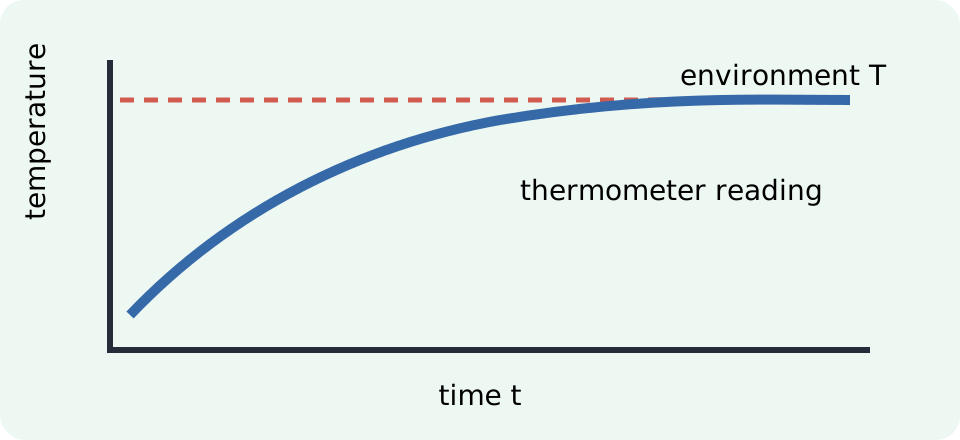
Response time depends on thermal resistance and thermal capacity. A simple first-order model is $T_{mathrm{th}}(t)=T_{mathrm{env}}+[T_{mathrm{th}}(0)-T_{mathrm{env}}]e^{-t/\tau}$. The symbol $\tau$ is the time constant, and after one $\tau$ the original difference falls to about $e^{-1}\approx0.368$ of its initial value. The thermometer approaches equilibrium asymptotically. Reading too early creates dynamic error.

Placement also matters. A surface probe, immersed probe, and infrared sensor can sample different physical regions. Temperature gradients make the phrase “the object’s temperature” ambiguous unless location is specified. Stirring can improve fluid uniformity but may add work or environmental exchange. Measurement design belongs to the scientific claim.

Repair common misconceptions

A common mistake is treating temperature as stored energy. Equal-temperature samples can have different masses, materials, phases, and internal energies. A small hot object can store less energy than a large cooler one. Temperature predicts thermal-transfer direction when systems interact. It does not by itself quantify total transferable energy.

Another mistake is averaging two temperatures without considering thermal capacities. The midpoint is correct only when the relevant $mc$ products are equal and no phase change or environmental transfer occurs. Write the energy balance before averaging. Include the container or thermometer when their capacities matter. Check that the final value lies within physically appropriate bounds.

A third mistake is using Celsius values in ratios or ideal-gas relations. Celsius and Kelvin share interval size but not zero. Convert coordinates to kelvins for absolute ratios and equations requiring thermodynamic temperature. A Celsius change can be used directly when only $\Delta T$ appears. Identify whether the formula uses a coordinate or an interval.

Practice with explanation

Convert $100.0\,^{\circ}\mathrm{C}$ to kelvins. The relation gives $T=100.0+273.15=373.15\,\mathrm{K}$. Appropriate final precision depends on the input convention. Explain why the kelvin value includes no degree symbol. Then explain why $100\,^{\circ}\mathrm{C}$ is not twice $50\,^{\circ}\mathrm{C}$ thermodynamically.

A $0.200\,\mathrm{kg}$ metal sample with $c=450\,\mathrm{\dfrac{J}{kg\,K}}$ at $100\,^{\circ}\mathrm{C}$ is placed with $0.500\,\mathrm{kg}$ water having $c=4180\,\mathrm{\dfrac{J}{kg\,K}}$ at $20.0\,^{\circ}\mathrm{C}$ in an ideal insulated container. The balance is $(0.200)(450)(T_f-100)+(0.500)(4180)(T_f-20.0)=0$ with consistent SI units. Solving gives approximately $T_f=23.3\,^{\circ}\mathrm{C}$. The result lies much closer to the water temperature because water has far greater thermal capacity. Identify what neglected container or environmental terms could alter the result.

A thermometer initially at $20.0\,^{\circ}\mathrm{C}$ is placed in an environment at $80.0\,^{\circ}\mathrm{C}$ with time constant $5.00\,\mathrm{s}$. After $5.00\,\mathrm{s}$, its reading is $80.0+(20.0-80.0)e^{-1}=57.9\,^{\circ}\mathrm{C}$. The thermometer has not yet reached equilibrium. After several time constants, the remaining difference becomes small. Explain how speed of response and measurement perturbation can create competing design goals.

Consolidate the temperature framework

Temperature is an intensive state variable defined operationally through thermal equilibrium and calibrated measurement. The zeroth law makes comparisons transitive and supports thermometer use. A temperature difference predicts the ordinary direction of spontaneous energy transfer by heating. Thermal equilibrium means no net thermal transfer, while steady state can preserve continuous through-flow. These distinctions anchor the subject macroscopically.

Kelvin is the SI thermodynamic scale, Celsius shares its interval size, and Fahrenheit uses a different interval and offset. Absolute ratios require kelvins. Equilibrium temperatures follow energy conservation and thermal capacities rather than unweighted averaging. Phase changes can alter internal energy at constant temperature. Measurement always carries response time, perturbation, and uncertainty.

Microscopic models enrich but do not replace the operational definition. For a monatomic ideal gas, temperature is proportional to mean translational kinetic energy, yet particles occupy a distribution of energies. Other systems include rotational, vibrational, potential, and quantum contributions. The next lesson will distinguish heat transfer from stored internal energy in greater detail. A careful definition of temperature prevents those concepts from collapsing into one another.