Exponential Functions

Linear change adds the same amount over equal input intervals, whereas exponential change multiplies by the same factor. That distinction is small in wording but profound in long-term behavior. Exponential models describe compound interest, radioactive decay, early population growth, drug elimination, and many other processes with approximately constant relative change. This lesson develops the meaning of every parameter before asking you to calculate with it. It also emphasizes evidence and model limitations so that a fitted curve is never mistaken for an unquestionable law.

Learning objectives and the multiplicative lens

By the end of this lesson, you will recognize exponential structure in formulas, tables, graphs, and contexts. You will interpret initial value, base, growth factor, percentage rate, and continuous rate with correct units. You will construct models from repeated change and from two observations. You will compute doubling time and half-life while keeping exponents dimensionless. You will also test whether an exponential model remains credible beyond the data used to build it.

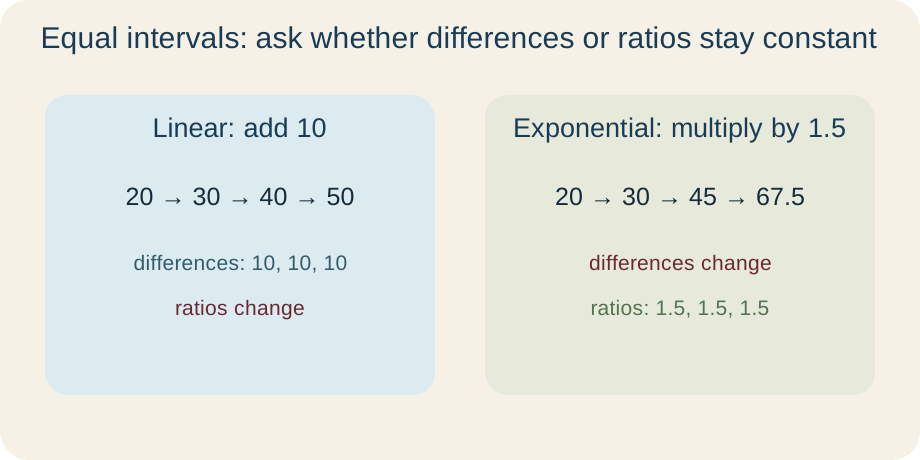
The central habit is to ask what remains constant. In a linear relationship, equal input steps produce equal output differences. In an exponential relationship, equal input steps produce equal output ratios. The ratio is multiplicative because one output is obtained by scaling the previous output. A constant ratio of $1.08$ means each new value is $108\%$ of the preceding value, not that eight fixed units are added.

Symbols should carry meaning rather than float free of context. In $Q(t)$, the letter $Q$ names the output quantity and $t$ names the input, often time. Parentheses in function notation mean “evaluate the rule at this input,” so $Q(3)$ is the output at input three. A superscript such as the $t$ in $b^t$ is an exponent, meaning the base $b$ is repeatedly scaled according to the input. The comparison diagram below makes the additive and multiplicative structures visible side by side.

Build the basic exponential model

The standard form is $f(x)=ab^x$, with $b>0$ and $b\ne1$. The coefficient $a$ is the initial value because $f(0)=ab^0=a$. The base $b$ is the factor associated with one unit of input. If $b>1$, positive values grow as $x$ increases. If $0<b<1$, positive values decay as $x$ increases.

Repeated multiplication explains why the input appears in the exponent. Starting from $a$, one interval produces $ab$, two intervals produce $ab^2$, and three intervals produce $ab^3$. After $n$ intervals, the value is $ab^n$. This reasoning first establishes the model for nonnegative integer inputs. Exponent rules extend it consistently to negative and fractional inputs when the context permits them.

The restrictions on $b$ protect the intended behavior. A zero base would make negative exponents undefined, while a negative base would prevent a real-valued output for many fractional inputs. The base $b=1$ gives the constant function $f(x)=a$, so it contains no growth or decay. The coefficient $a$ may be negative in pure mathematics, but many applications such as mass or population require $a>0$. Always derive contextual restrictions separately from the mathematical domain.

Translate rates into factors

A decimal rate $r$ per interval corresponds to the growth factor $b=1+r$. The number $1$ represents the entire current amount, and $r$ represents the added fraction of that amount. A $6\%$ growth rate is $r=0.06$, so the factor is $1.06$. Multiplying by $1.06$ retains the original $100\%$ and adds $6\%$. Entering $6$ instead of $0.06$ would incorrectly represent $600\%$.

For decay at rate $r$, the remaining factor is $b=1-r$. A $6\%$ decay rate leaves $94\%$, so $b=0.94$. The decay rate is not the same object as the remaining factor. If a quantity is multiplied by $0.72$ each hour, it retains $72\%$ and loses $28\%$ each hour. Subtracting the factor from one recovers the decay rate.

Percentage increases and decreases of equal size do not undo one another. If a value grows by $20\%$ and then falls by $20\%$, the combined factor is $(1.20)(0.80)=0.96$. The final value is $96\%$ of the original, so the net change is a $4\%$ loss. The asymmetry occurs because the decrease acts on the already increased amount. Compound factors must be multiplied in the order of the changes, although multiplication makes the final product independent of order.

Identify exponential evidence in tables and graphs

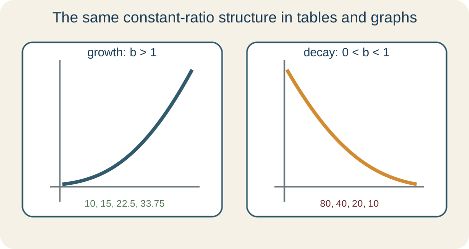
For equal input increments, compute successive output ratios. The outputs $40$, $60$, $90$, and $135$ have common ratio $1.5$, so they follow an exponential pattern over those steps. Their first differences are $20$, $30$, and $45$, which are not constant. By contrast, the outputs $40$, $60$, $80$, and $100$ have constant difference $20$ and are linear. A table can therefore distinguish the two structures without a graph.

For $f(x)=ab^x$, an input step of size $h$ gives $\frac{f(x+h)}{f(x)}=b^h$. The horizontal fraction bar means the later output is divided by the earlier output. The result does not depend on $x$, which expresses constant relative change over equal intervals. If table inputs differ by two units rather than one, the observed ratio is $b^2$, not $b$. Taking an appropriate root recovers the factor per single input unit.

With $a>0$, an exponential graph stays above the horizontal axis and has $y=0$ as a horizontal asymptote. An asymptote is a line the graph approaches in an end behavior, not a barrier defined by drawing convention. For growth, the curve rises increasingly steeply to the right and approaches zero to the left. For decay, those directions reverse. The point $(0,a)$ is the vertical-axis intercept and anchors every graph in standard form.

Model discrete compound growth

Suppose an account begins with $1{,}500\,\mathrm{dollars}$ and earns $4.0\%$ once each year. The annual factor is $1.04$, so $A(t)=1{,}500\,\mathrm{dollars}(1.04)^{t/(1\,\mathrm{year})}$. Writing $t/(1\,\mathrm{year})$ makes the exponent dimensionless. After $6.0\,\mathrm{years}$, the exponent is six. The model gives approximately $1{,}898\,\mathrm{dollars}$ after rounding to the nearest dollar.

If interest is compounded $n$ times per year at nominal annual rate $r$, the model is $A(t)=P\left(1+\frac{r}{n}\right)^{nt}$. The symbol $P$ is the principal, meaning the initial balance. The fraction $\frac{r}{n}$ is the rate per compounding period, and $nt$ counts the periods when $t$ is measured in years. Monthly compounding uses $n=12$, while daily textbook models often use $n=365$. The stated convention must match the application.

A nominal rate is not automatically the actual one-year percentage increase. At nominal rate $r=0.06$ compounded monthly, the one-year factor is $\left(1+\frac{0.06}{12}\right)^{12}$. Subtracting one from that factor gives the effective annual rate. More frequent compounding produces a slightly larger effective rate when the nominal rate is positive. Financial contexts may also include fees, deposits, and changing rates that require a more detailed model.

Connect discrete and continuous growth

Continuous exponential change is written $Q(t)=Q_0e^{kt}$. The constant $e$ is approximately $2.71828$ and is the natural base for continuously compounded change. The parameter $k$ is the continuous relative growth constant. If $k>0$, the quantity grows, and if $k<0$, it decays. When $t$ carries time units, $k$ must carry reciprocal-time units.

Discrete and continuous parameters describe the same one-unit factor in different languages. If $b^t=e^{kt}$ for the same time unit, then $b=e^k$ and $k=\ln b$. The symbol $\ln$ denotes the natural logarithm, which reverses exponentiation with base $e$. A $5\%$ discrete annual factor is $b=1.05$, so the corresponding continuous constant is $k=\ln(1.05)$ per year. The numerical value of $k$ is about $0.04879\,\mathrm{year}^{-1}$, not exactly $0.05\,\mathrm{year}^{-1}$.

The equation $Q'=kQ$ explains why continuous exponentials appear in differential equations. The prime means derivative with respect to time, so $Q'$ is the instantaneous rate of change. Dividing by $Q$ gives $\frac{Q'}{Q}=k$, a constant relative rate. The solution $Q(t)=Q_0e^{kt}$ is the function whose derivative is always $k$ times itself. This calculus connection formalizes the idea that the rate is proportional to the current amount.

Interpret doubling time and half-life

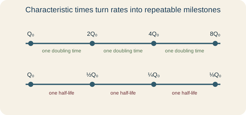
For $Q(t)=Q_0e^{kt}$ with $k>0$, the doubling time $T_2$ satisfies $Q(T_2)=2Q_0$. Canceling the nonzero initial value gives $e^{kT_2}=2$. Applying the natural logarithm yields $kT_2=\ln 2$. Therefore $T_2=\frac{\ln 2}{k}$. Its units are time because the reciprocal of $k$ carries time units.

For decay with $k<0$, the half-life $T_{1/2}$ satisfies $Q(T_{1/2})=\frac{1}{2}Q_0$. Solving gives $T_{1/2}=\frac{\ln 2}{|k|}$, where vertical bars denote absolute value. The absolute value makes the denominator positive because a duration must be positive. A larger magnitude of $k$ means faster decay and a shorter half-life. Half-life remains constant in a pure exponential model regardless of the current amount.

A sample with initial mass $80\,\mathrm{mg}$ and half-life $6\,\mathrm{h}$ has model $M(t)=80\,\mathrm{mg}\left(\frac{1}{2}\right)^{t/(6\,\mathrm{h})}$. After $18\,\mathrm{h}$, the dimensionless exponent is three. Three halvings leave $10\,\mathrm{mg}$. This computation does not mean individual atoms carry timers; radioactive decay describes predictable ensemble behavior. Measurement uncertainty and background radiation still matter in real experiments.

Estimate a model from observations

Suppose $Q(t)=Q_0b^{t/(1\,\mathrm{year})}$ and measurements give $Q(0)=200\,\mathrm{units}$ and $Q(3\,\mathrm{years})=266.2\,\mathrm{units}$. The total three-year factor is $\frac{266.2}{200}=1.331$. The annual factor is the cube root, $b=(1.331)^{1/3}=1.10$. Therefore the annual growth rate is $10\%$. Using $1.331$ as the annual factor would confuse total change with per-interval change.

When neither observation occurs at time zero, ratios still eliminate the unknown initial coefficient. If $Q(t_1)=Q_1$ and $Q(t_2)=Q_2$, then $\frac{Q_2}{Q_1}=b^{(t_2-t_1)/(1\,\mathrm{time\ unit})}$. The elapsed time is $t_2-t_1$, not simply $t_2$. Solving for $b$ gives the factor per chosen time unit. Substituting either observation then determines the coefficient for the selected time origin.

Real measurements rarely produce perfectly constant ratios. One can transform a positive exponential model using $\ln Q(t)=\ln Q_0+kt$, which is linear in time. A roughly straight plot of $ln Q$ against $t$ supports the exponential hypothesis. However, fitting on a logarithmic scale changes how errors are weighted and requires positive observations. Residual plots should still be inspected to find systematic deviations.

Respect domains, units, and model limits

The mathematical domain of $ab^x$ is all real $x$ when $b>0$, but a context can narrow it. Annual deposits made at discrete times may permit integer inputs only. A population count cannot be negative even if an extrapolated formula remains positive. A medication model may apply only after absorption and before another dose. State the contextual domain alongside the equation.

Every exponent must be dimensionless. In $e^{kt}$, this happens because inverse-time units in $k$ cancel time units in $t$. In a half-life model, $t/T_{1/2}$ is a ratio of two times and therefore has no units. Changing hours to days changes numerical parameter values but not the physical prediction. A model that places a dimensional quantity directly in an exponent is incomplete until a scale makes the ratio unitless.

Pure exponential growth assumes a constant relative rate and no limiting capacity. Populations may approximate it only while resources remain abundant, and financial models may fail when rates change. Radioactive decay is often exceptionally close to exponential at the ensemble level, yet measurement and contamination can distort small samples. Extrapolation far beyond observed inputs increases risk because tiny rate errors compound. A good model report names both the useful range and the mechanisms that may break the assumption.

Guided practice and error analysis

Model $800$ bacteria increasing by $12\%$ per hour. The initial value is $800\,\mathrm{bacteria}$ and the hourly factor is $1.12$. A unit-explicit model is $N(t)=800\,\mathrm{bacteria}(1.12)^{t/(1\,\mathrm{h})}$. After $5\,\mathrm{h}$, it predicts approximately $1{,}410\,\mathrm{bacteria}$. Because actual counts are integers, round only after evaluating the continuous-valued model.

Now consider $Q(t)=50\,\mathrm{g}(0.8)^{t/(1\,\mathrm{day})}$. The factor $0.8$ means $80\%$ remains each day, so $20\%$ is lost. It does not mean the quantity loses $0.8\,\mathrm{g}$ per day. After two days the value is $50\,\mathrm{g}(0.8)^2=32\,\mathrm{g}$. The daily losses are $10\,\mathrm{g}$ and $8\,\mathrm{g}$, demonstrating that equal percentages create unequal absolute changes.

For independent synthesis, a medicine begins at $120\,\mathrm{mg}$ and has half-life $8\,\mathrm{h}$. Write a dimensionally correct model, predict the amount after $20\,\mathrm{h}$, and identify the contextual domain. Explain the meaning of the base, exponent, and initial coefficient in complete sentences. Then state at least two biological mechanisms that could make a one-compartment exponential model inaccurate. Check that the predicted amount is positive and less than the initial amount.

Synthesis and connection forward

Exponential functions encode constant multiplicative change over equal intervals. Initial value locates the model, the base gives a discrete factor, and a continuous constant gives an instantaneous relative rate. Tables reveal equal ratios, graphs reveal characteristic curvature and asymptotes, and equations make prediction possible. Doubling time and half-life translate rates into intuitive time scales. Units and dimensionless exponents keep every representation coherent.

The strongest modeling workflow moves from mechanism to equation and then back to evidence. Decide whether repeated proportional change is plausible, define the variables and their units, estimate parameters, and compare predictions with observations. Inspect residuals instead of relying only on visual resemblance. Restrict the domain to the setting where assumptions remain defensible. Communicate uncertainty whenever parameters come from measured data.

Logarithms provide the inverse operation needed when the unknown appears in an exponent. They answer questions such as how long a balance takes to double or when a drug level crosses a threshold. Sequences formalize discrete exponential steps, while differential equations formalize continuous proportional change. Logistic models modify the exponential rule when capacity limits growth. The concepts in this lesson therefore connect algebraic functions to statistics, calculus, and applied science.