Entropy and the Second Law

Some processes have a natural direction even though energy is conserved in either direction. A hot object cools in a cooler room, gases mix after a partition is removed, and a dropped object’s organized mechanical energy becomes dispersed thermal energy. The reverse events do not violate the first law, yet they are not observed as spontaneous macroscopic changes. Entropy and the second law supply the missing directional criterion. They explain how energy and matter distribute among the microscopic possibilities compatible with a macroscopic state.

You will connect entropy to microstates, interpret thermal entropy transfer, predict signs for phase and mixing changes, calculate standard reaction entropy, and include the surroundings. You will distinguish a spontaneous process from a fast process and explain why a system’s entropy may decrease while the total still increases. The notation $S$, $\Delta S$, $k_{\mathrm B}$, $\Omega$, and $q_{\mathrm{rev}}$ will be defined before it is used. Examples will preserve kelvin and joule units in horizontal fractional form. The goal is a conservation-and-probability framework, not the slogan that entropy means “disorder.”

Approach every problem by defining the system, surroundings, initial state, final state, and constraints. Ask whether the process changes the number or distribution of accessible microscopic arrangements. Then determine entropy changes for both system and surroundings rather than judging the system alone. Use qualitative trends when only a sign is requested and quantitative data when available. Finally separate thermodynamic direction from kinetic rate.

Macrostates summarize many microscopic arrangements

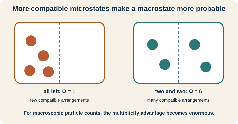
A macrostate is described by bulk variables such as temperature, pressure, volume, and composition. A microstate specifies microscopic details consistent with those bulk measurements, including particle positions and energy allocations. Many distinct microstates can look identical at macroscopic resolution. The symbol $\Omega$, the Greek capital omega, denotes the number of microstates compatible with a chosen macrostate. A macrostate with larger $\Omega$ has more microscopic ways to occur.

Imagine four distinguishable particles distributed between equal left and right compartments. There is only one positional arrangement with all four on the left, but six arrangements with two on each side because different pairs can occupy the left. If every accessible positional microstate is equally likely, the evenly divided macrostate is more probable than the all-left macrostate. With a mole of particles, the numerical advantage of broadly distributed states becomes overwhelming. The spontaneous direction reflects this multiplicity rather than a rule imposed on each particle.

The word “disorder” can be suggestive in simple illustrations, but it is not a rigorous definition. A shuffled deck may look disordered to a person, yet entropy requires a physical model of accessible states and constraints. A crystal may have positional regularity while still possessing thermal vibrational microstates. Mixing may raise entropy even when the mixture appears visually uniform and orderly. Focus on multiplicity and energy dispersal instead of aesthetic judgments.

Boltzmann’s relation makes multiplicity quantitative

Boltzmann’s relation is $S=k_{\mathrm B}\ln\Omega$. The symbol $S$ denotes entropy, $k_{\mathrm B}$ is Boltzmann’s constant, $\ln$ is the natural logarithm, and $\Omega$ is compatible microstate count. Boltzmann’s constant has units $\frac{\mathrm{J}}{\mathrm{K}}$, so entropy also has units joules per kelvin. The logarithm turns multiplication of independent multiplicities into addition of entropies. This additivity makes entropy an extensive thermodynamic property.

For two independent subsystems, the combined microstate count is $\Omega_{\text{total}}=\Omega_1\Omega_2$. Applying the logarithm gives $S_{\text{total}}=k_{\mathrm B}\ln(\Omega_1\Omega_2)=k_{\mathrm B}\ln\Omega_1+k_{\mathrm B}\ln\Omega_2$. Thus $S_{\text{total}}=S_1+S_2$. Doubling the amount of similar material approximately doubles its entropy at the same state. The logarithmic form connects enormous microscopic counts to manageable macroscopic values.

Entropy change between two macrostates can be written $\Delta S=k_{\mathrm B}\ln\left(\frac{\Omega_f}{\Omega_i}\right)$. The subscripts $f$ and $i$ denote final and initial states. If $\Omega_f>\Omega_i$, the logarithm is positive and entropy increases. If the final state has fewer accessible microstates, the entropy change is negative. This equation makes the direction of the change explicit without treating entropy as a substance that physically fills space.

Thermal entropy transfer depends on temperature

For a reversible transfer of an infinitesimal heat amount, $dS=\frac{\delta q_{\mathrm{rev}}}{T}$. The symbol $dS$ represents an infinitesimal change in the state function entropy. The symbol $\delta q_{\mathrm{rev}}$ represents infinitesimal heat transferred along a reversible path; the different symbol emphasizes that heat is path dependent rather than a state function. The denominator $T$ is absolute temperature in kelvins. Dividing joules by kelvins gives the entropy unit $\frac{\mathrm{J}}{\mathrm{K}}$.

For a reversible isothermal process at constant temperature, integration gives $\Delta S=\frac{q_{\mathrm{rev}}}{T}$. The equation does not say entropy equals heat. The same heat transfer produces a larger entropy change at a lower temperature because that energy constitutes a larger relative redistribution among available modes. Temperature must be expressed in kelvins because the thermodynamic scale begins at absolute zero. A Celsius value cannot be substituted directly into the denominator.

Real spontaneous processes are irreversible, but entropy change depends only on initial and final equilibrium states. One may therefore calculate $\Delta S$ by imagining any convenient reversible path between the same endpoints. The actual irreversible path need not be reproducible in reverse without net changes elsewhere. This strategy separates the state-function calculation from the physical path. It also explains why the subscript “rev” belongs to the heat quantity in the calculation rather than claiming the actual process was reversible.

The second law applies to system plus surroundings

The entropy statement of the second law is $\Delta S_{\text{total}}\ge 0$ for an isolated total system. Here $\Delta S_{\text{total}}=\Delta S_{\text{sys}}+\Delta S_{\text{surr}}$, where “sys” means the chosen system and “surr” means its surroundings. A spontaneous irreversible process has $\Delta S_{\text{total}}>0$. An ideal reversible process has $\Delta S_{\text{total}}=0$. A proposed process with negative total entropy change cannot occur spontaneously under the stated constraints.

The system’s entropy alone need not increase. Water can freeze below its freezing temperature even though the liquid-to-solid change decreases the water’s entropy. Heat released to the colder surroundings can increase the surroundings’ entropy by a larger amount. The total then remains positive, satisfying the second law. Defining the boundary prevents the false claim that every local region must become more dispersed.

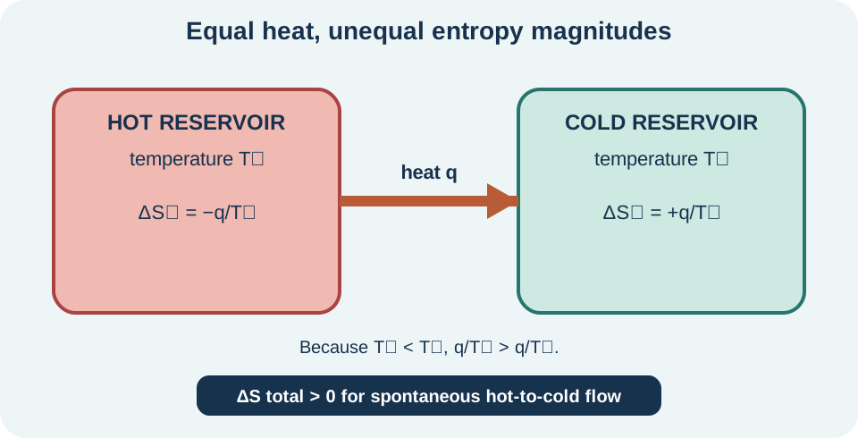
For heat transfer from a hot reservoir at temperature $T_h$ to a cold reservoir at $T_c$, let a positive heat magnitude $q$ leave the hot side and enter the cold side. The hot entropy change is $\Delta S_h=-\frac{q}{T_h}$, while the cold change is $\Delta S_c=\frac{q}{T_c}$. Because $T_c<T_h$, the positive magnitude $\frac{q}{T_c}$ exceeds the negative magnitude $\frac{q}{T_h}$. Their sum is positive, explaining the spontaneous hot-to-cold direction. Reversing the transfer would make the modeled total change negative.

Phase changes reveal accessible-state differences

Entropy generally increases along the progression solid to liquid to gas for a given substance at comparable conditions. In a solid, particles are localized around lattice positions while retaining vibrational motion. In a liquid, particles can rearrange and translate through the sample. In a gas, positions and energy distributions span a much larger accessible volume. These statements describe changes in accessible microstates rather than visual messiness.

At a phase-transition temperature where two phases coexist reversibly, the entropy change is $\Delta S_{\text{trans}}=\frac{\Delta H_{\text{trans}}}{T_{\text{trans}}}$. The subscript “trans” denotes the phase transition, such as fusion or vaporization. For vaporization, $\Delta H_{\text{vap}}$ is positive and the entropy change of the substance is positive. Condensation reverses both signs. Units of $\frac{\mathrm{J}}{\mathrm{mol}}$ divided by kelvins give $\frac{\mathrm{J}}{\mathrm{mol\,K}}$.

Consider water vaporizing at $373.15\,\mathrm{K}$ with a molar enthalpy of vaporization near $40.7\,\frac{\mathrm{kJ}}{\mathrm{mol}}$. Convert kilojoules to joules before combining with entropy units: $40.7\,\frac{\mathrm{kJ}}{\mathrm{mol}}=4.07\times10^4\,\frac{\mathrm{J}}{\mathrm{mol}}$. Then $\Delta S_{\text{vap}}=\frac{4.07\times10^4\,\frac{\mathrm{J}}{\mathrm{mol}}}{373.15\,\mathrm{K}}\approx109\,\frac{\mathrm{J}}{\mathrm{mol\,K}}$. The positive result agrees with the much larger positional freedom of gas. The calculation applies at the reversible coexistence temperature.

Chemical trends are useful but conditional

Several qualitative trends help predict the sign of a system entropy change. Producing more moles of gas from fewer moles of gas often increases entropy. Mixing distinguishable gases or dissolved species usually increases entropy because more distributions become accessible. Dissolving a crystalline solid may increase entropy through dispersal, but strong solvation organization can oppose that trend. Raising temperature generally increases a substance’s entropy by making more energy levels accessible.

These are tendencies rather than proofs. The reaction $\mathrm{2SO_2(g)+O_2(g)\longrightarrow2SO_3(g)}$ reduces gas amount from three stoichiometric moles to two and therefore suggests negative system entropy change. Yet precise prediction should use tabulated molar entropies because molecular complexity and state conditions also contribute. A single phrase such as “fewer particles” does not quantify all degrees of freedom. Use structural trends to anticipate a sign, then calculate when data are supplied.

State symbols are indispensable. Converting one mole of liquid water to one mole of gaseous water changes entropy substantially even though chemical formulas and stoichiometric amount remain the same. Similarly, dissolving an ionic solid changes how particles occupy solvent environments. A reaction equation without $\mathrm{(s)}$, $\mathrm{(l)}$, $\mathrm{(g)}$, and $\mathrm{(aq)}$ labels omits information needed for entropy reasoning. Always read physical states before counting species.

Calculate standard reaction entropy

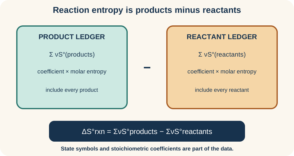
The standard reaction entropy is $\Delta S^\circ_{\mathrm{rxn}}=\sum \nu S^\circ_{\mathrm{products}}-\sum \nu S^\circ_{\mathrm{reactants}}$. The superscript degree symbol denotes standard-state conditions, $\nu$ represents stoichiometric coefficient, and $S^\circ$ is standard molar entropy. The Greek capital sigma $\sum$ instructs you to add the coefficient-weighted terms in each group. Products are summed first and the reactant sum is subtracted. Units are typically $\frac{\mathrm{J}}{\mathrm{mol\,K}}$ per mole of reaction as written.

Suppose a reaction is $\mathrm{A(g)+2B(g)\longrightarrow C(g)}$ with standard molar entropies $S_A^\circ=200\,\frac{\mathrm{J}}{\mathrm{mol\,K}}$, $S_B^\circ=150\,\frac{\mathrm{J}}{\mathrm{mol\,K}}$, and $S_C^\circ=250\,\frac{\mathrm{J}}{\mathrm{mol\,K}}$. The product sum is $1(250)=250\,\frac{\mathrm{J}}{\mathrm{mol\,K}}$. The reactant sum is $1(200)+2(150)=500\,\frac{\mathrm{J}}{\mathrm{mol\,K}}$. Therefore $\Delta S^\circ_{\mathrm{rxn}}=250-500=-250\,\frac{\mathrm{J}}{\mathrm{mol\,K}}$. The negative sign means the reaction system has fewer accessible arrangements in this comparison.

The negative result is consistent with three stoichiometric moles of gas becoming one in the simplified reaction. Coefficients must multiply entropy values because entropy is extensive. Elements in their standard states do not have zero standard molar entropy at ordinary temperature, unlike standard enthalpies of formation. The third law assigns zero entropy only to a perfect crystal at absolute zero under its ideal assumptions. Confusing these reference conventions produces systematic reaction-entropy errors.

The surroundings entropy connects heat and direction

At constant pressure, heat exchanged by the system is related to its enthalpy change, and the surroundings receive the opposite heat. If the surroundings remain at constant temperature $T$, a common model is $\Delta S_{\text{surr}}=-\frac{\Delta H_{\text{sys}}}{T}$. An exothermic system has $\Delta H_{\text{sys}}<0$, making $\Delta S_{\text{surr}}>0$. An endothermic system has $\Delta H_{\text{sys}}>0$, making the surroundings entropy change negative. The sign reflects heat leaving or entering the surroundings.

Suppose a reaction releases $50.0\,\frac{\mathrm{kJ}}{\mathrm{mol}}$ at $298\,\mathrm{K}$. Write the system enthalpy as $-50.0\,\frac{\mathrm{kJ}}{\mathrm{mol}}=-5.00\times10^4\,\frac{\mathrm{J}}{\mathrm{mol}}$. Then $\Delta S_{\text{surr}}=-\frac{-5.00\times10^4\,\frac{\mathrm{J}}{\mathrm{mol}}}{298\,\mathrm{K}}=+168\,\frac{\mathrm{J}}{\mathrm{mol\,K}}$ to three significant figures. Converting kilojoules to joules is necessary before adding this result to a system entropy expressed in joules per mole-kelvin. The positive value records heat gained by the surroundings.

If the reaction’s system entropy change were $-120\,\frac{\mathrm{J}}{\mathrm{mol\,K}}$, the modeled total would be $+48\,\frac{\mathrm{J}}{\mathrm{mol\,K}}$. The system becomes less dispersed, but the surroundings gain more entropy than the system loses. The total positive value predicts spontaneity under the stated conditions. A local entropy decrease and a spontaneous overall process are therefore fully compatible. The system boundary is what makes the two statements coexist without contradiction.

Gibbs energy packages the constant-temperature criterion

At constant temperature and pressure, Gibbs free-energy change is $\Delta G=\Delta H-T\Delta S_{\text{sys}}$. The product $T\Delta S$ has energy units because kelvins multiply joules per kelvin. A process is thermodynamically spontaneous in the forward direction under the stated conditions when $\Delta G<0$. At equilibrium, $\Delta G=0$. A positive value favors the reverse direction rather than proving that no reaction molecules ever form.

The criterion follows from total entropy when the surroundings act as a thermal reservoir. Using $\Delta S_{\text{surr}}=-\frac{\Delta H_{\text{sys}}}{T}$ gives $\Delta S_{\text{total}}=\Delta S_{\text{sys}}-\frac{\Delta H_{\text{sys}}}{T}$. Multiplying by $-T$ yields $-T\Delta S_{\text{total}}=\Delta H_{\text{sys}}-T\Delta S_{\text{sys}}=\Delta G$. Since $T$ is positive on the kelvin scale, positive total entropy corresponds to negative Gibbs energy. The two criteria describe the same direction under the relevant constraints.

Temperature can change spontaneity when enthalpy and entropy contributions compete. If both $\Delta H$ and $\Delta S$ are positive, the enthalpy term opposes spontaneity while the $-T\Delta S$ term favors it increasingly at high temperature. If both are negative, low temperature can favor the negative enthalpy term while high temperature magnifies the unfavorable entropy term. The equation must be applied with consistent units and realistic temperature dependence. Sign tables are summaries of this balance, not replacements for it.

Spontaneous does not mean fast

Thermodynamics predicts direction and equilibrium tendency, while kinetics describes rate and mechanism. Diamond transforming to graphite is thermodynamically favorable under ordinary conditions, yet the process is extremely slow because bonds must reorganize through a high activation barrier. Combustible mixtures may remain unchanged until a spark supplies activation energy. A negative Gibbs energy does not eliminate the kinetic pathway requirement. It states the energetic direction once the process can proceed.

A catalyst speeds forward and reverse reaction pathways by lowering activation barriers. It does not change $\Delta S$, $\Delta G$, or the equilibrium constant for the same temperature. Therefore a catalyst helps a system approach equilibrium sooner without changing the equilibrium composition. This distinction prevents rate observations from being used as direct measures of thermodynamic favorability. Fast can be unfavorable in a driven context, and favorable can be imperceptibly slow.

The words spontaneous and instantaneous should never be treated as synonyms. “Spontaneous” means that the total entropy criterion favors the direction under specified constraints. A process may still require a finite fluctuation or initiation event. Its observed timescale depends on molecular collisions, pathway geometry, activation energy, and transport. Always answer direction and rate as separate questions.

Common misconceptions and corrective habits

One misconception states that the entropy of everything always increases at every moment. The second law concerns total entropy for an isolated whole and allows local decreases when compensated elsewhere. Define the system and surroundings before assigning signs. Another misconception says exothermic reactions are always spontaneous. An unfavorable system entropy change can overcome enthalpy at some temperatures.

A second misconception equates entropy with visible messiness. Visual order is observer dependent, whereas entropy follows accessible microstates under physical constraints. Use phase, volume, energy levels, mixing, and molecular degrees of freedom to justify a trend. A third misconception sets the standard entropy of an element to zero. That zero convention belongs to standard enthalpy of formation, not standard molar entropy at ordinary temperature.

A numerical error often arises from mixing kilojoules and joules. Entropy data are commonly tabulated in $\frac{\mathrm{J}}{\mathrm{mol\,K}}$, while enthalpy is commonly in $\frac{\mathrm{kJ}}{\mathrm{mol}}$. Convert before adding $\Delta S_{\text{sys}}$ and $\Delta S_{\text{surr}}$ or before evaluating $T\Delta S$. Keep temperature in kelvins and write every unit through cancellation. Dimensional consistency is an essential final check.

Guided practice and retrieval

Predict the sign of entropy change when one mole of liquid ethanol vaporizes at its boiling point. The gas phase provides much greater positional freedom than the liquid, so the system entropy change is positive. The reversible phase-transition relationship is $\Delta S_{\text{vap}}=\frac{\Delta H_{\text{vap}}}{T_b}$, where $T_b$ is boiling temperature in kelvins. Both numerator and denominator must use compatible energy and temperature units. Condensation would reverse the sign.

A system absorbs $12.0\,\frac{\mathrm{kJ}}{\mathrm{mol}}$ from surroundings at $300\,\mathrm{K}$. The surroundings entropy change is $-\frac{1.20\times10^4\,\frac{\mathrm{J}}{\mathrm{mol}}}{300\,\mathrm{K}}=-40.0\,\frac{\mathrm{J}}{\mathrm{mol\,K}}$. If the system entropy rises by $65.0\,\frac{\mathrm{J}}{\mathrm{mol\,K}}$, the total change is $+25.0\,\frac{\mathrm{J}}{\mathrm{mol\,K}}$. The modeled direction is spontaneous because total entropy is positive. Explain why the endothermic sign alone was insufficient.

Finally, compare free expansion of a gas into an evacuated chamber with spontaneous heat flow. In expansion, a larger accessible volume increases positional microstates even if ideal-gas energy remains unchanged. In heat flow, the same energy becomes more broadly distributed between bodies, producing a positive total entropy change. Both processes illustrate movement toward overwhelmingly more numerous macrostates. Neither should be explained merely by saying “nature likes disorder.” Name the changed constraint in each case to complete the explanation.

Connection forward

Reconstruct the lesson’s reasoning without looking back. Define macrostate, microstate, multiplicity, system, surroundings, reversible path, and spontaneous direction. Explain $S=k_{\mathrm B}\ln\Omega$, $\Delta S_{\text{total}}\ge0$, and $\Delta S_{\text{surr}}=-\frac{\Delta H_{\text{sys}}}{T}$ in words and units. State why system entropy can decrease during a spontaneous process. Then separate that thermodynamic conclusion from any claim about rate.

The Gibbs free-energy lesson will compress system and surroundings effects into a practical constant-temperature, constant-pressure criterion. Equilibrium constants will connect standard Gibbs energy to the composition favored at equilibrium. Phase equilibria will use chemical potentials and entropy changes to locate transitions. Kinetics will explain how barriers and mechanisms determine whether thermodynamic tendencies are observable on a chosen timescale. Each topic preserves the same distinction between direction, extent, and speed.

The enduring picture is probabilistic but not arbitrary. Macroscopic systems evolve toward distributions supported by overwhelmingly more accessible microscopic arrangements, while energy and matter remain conserved. Entropy quantifies that multiplicity and thermal dispersal, and the second law applies the criterion to the complete isolated whole. Local organization can arise when its surroundings pay a larger entropy cost. With boundaries, units, and constraints explicit, entropy becomes an accounting framework rather than a mysterious synonym for disorder.