The Second Law and Entropy

The first law requires energy accounting to balance. It does not say which energy transfers happen spontaneously. A hot object warms a cold object, yet the reverse transfer would also conserve energy. A gas expands into an available volume but does not ordinarily gather itself back into one side. The second law distinguishes allowed direction from mere energy conservation.

Entropy is the state quantity used in that distinction. It tracks how energy and microscopic possibilities are distributed, while entropy generation measures irreversibility. Entropy can move across a system boundary with heat and matter. It can also be generated inside a system. Unlike energy, it is not conserved.

This lesson connects macroscopic balances, heat transfer, reversible limits, engines, refrigerators, and statistical interpretation. It uses kelvins, joules, and joules per kelvin explicitly. It avoids treating entropy as a synonym for “disorder.” Three diagrams organize the ledgers and device flows. The aim is to understand what the second law permits, forbids, and quantifies.

Learning goals and a direction puzzle

You should distinguish first-law and second-law questions. You should calculate entropy changes for reservoirs and reversible paths. You should write system and universe entropy balances. You should explain entropy generation and reversible limits. You should derive and apply the Carnot efficiency bound.

Place a hot metal block in contact with a colder block inside an insulated container. Energy lost by the hot block equals energy gained by the cold block. The first-law total is zero in either imagined transfer direction. Experience nevertheless selects heat flow from hot to cold. Entropy change selects the same direction.

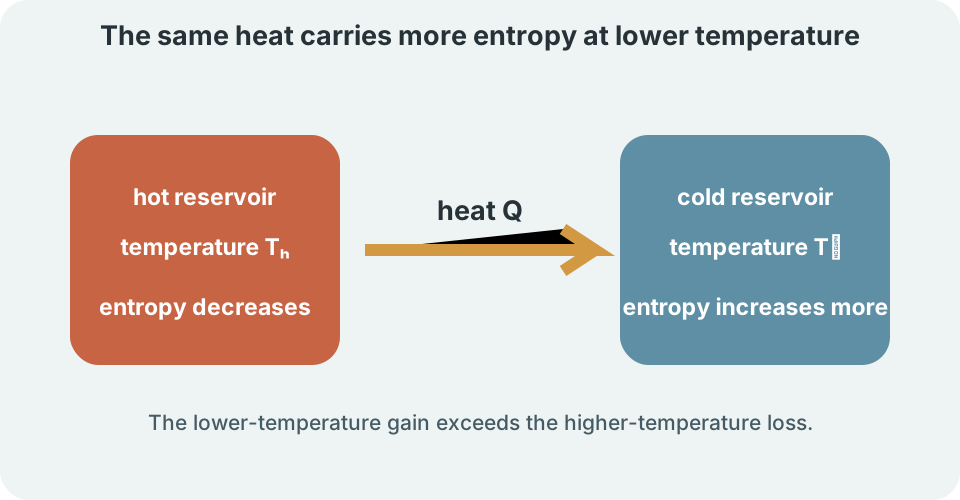
Predict whether the hot block’s entropy increases. It loses heat, so its entropy decreases. The cold block’s entropy increases by a greater amount because the same energy arrives at lower absolute temperature. Their sum is positive. A subsystem can decrease in entropy while the isolated whole increases.

The first law is necessary but insufficient

For a closed system under one common sign convention, $\Delta U=Q-W$. Internal-energy change $\Delta U$ equals heat $Q$ transferred into the system minus work $W$ done by the system. The equation balances energy quantity. It does not attach a direction test to a proposed process. Both signs must follow a declared convention.

Consider converting mechanical work entirely into thermal energy by friction. The first law permits it and experience confirms it. The reverse process would convert random thermal motion entirely into organized macroscopic work with no other change. Energy could still balance. The second law rules out that cyclic outcome.

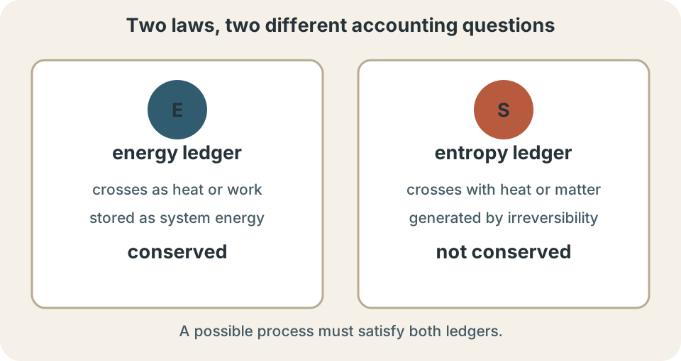
Thermodynamic analysis therefore needs two ledgers. The energy ledger asks where energy goes. The entropy ledger asks whether a proposed direction requires negative total entropy generation. A process must satisfy both. Passing one law does not excuse failing the other.

Entropy is a state function

Entropy is represented by $S$. It is a state function, so its change depends only on initial and final equilibrium states. The path affects heat and work but not the state difference $\Delta S=S_f-S_i$. Different processes connecting the same states have the same system entropy change. This permits a reversible calculation path for an irreversible process.

The SI unit of entropy is $\mathrm{\frac{J}{K}}$. Joules measure energy, and kelvins measure absolute temperature. Entropy change per unit mass may use $\mathrm{\frac{J}{kg\,K}}$. Molar entropy may use $\mathrm{\frac{J}{mol\,K}}$. Units must match the chosen amount basis.

Entropy is extensive. Doubling an otherwise identical system doubles its entropy. Specific entropy and molar entropy are intensive because amount has been divided out. A value without system size or basis can be ambiguous. State labels and units make the quantity interpretable.

Reversible heat defines entropy change

For an infinitesimal reversible heat transfer, $dS=\frac{\delta Q_{\mathrm{rev}}}{T}$. Differential $dS$ marks an exact state-function differential. Symbol $\delta Q$ reminds us that heat is a path transfer rather than stored state content. Subscript “rev” identifies a reversible path. Temperature $T$ must be absolute.

For a finite change, integrate: $\Delta S=\int_i^f\frac{\delta Q_{\mathrm{rev}}}{T}$. If the reversible transfer occurs at constant temperature, this becomes $\Delta S=\frac{Q_{\mathrm{rev}}}{T}$. The horizontal fraction divides transferred energy by absolute temperature. Its unit is $\mathrm{\frac{J}{K}}$. Integration adds contributions along the reversible path.

The equation does not claim a real irreversible process has a well-defined boundary temperature at every moment. Instead, choose any convenient reversible path between the same states to calculate system entropy change. Entropy generation is then determined from the actual process balance. Reversible path and real path must not be conflated. They share endpoints but not mechanisms.

Kelvin temperature is essential

Entropy formulas divide by absolute temperature. Kelvin zero represents the absolute lower limit in the thermodynamic scale. Celsius zero is an arbitrary reference associated with water. Ratios such as $\frac{T_c}{T_h}$ make physical sense only on an absolute scale. Celsius values cannot be inserted directly.

Convert with $T_{\mathrm K}=T_{^\circ\mathrm C}+273.15$. A temperature of $27.0\,^\circ\mathrm C$ is $300.15\,\mathrm K$. A temperature difference of $10\,^\circ\mathrm C$ equals a difference of $10\,\mathrm K$. Absolute values and differences follow different conversion behavior. Entropy formulas require the absolute value.

Using Celsius in $\frac{Q}{T}$ can reverse trends or create division by zero at $0\,^\circ\mathrm C$. That failure is not a minor unit preference. It violates the structure of thermodynamic temperature. Write kelvin units in every entropy and Carnot calculation. Unit discipline protects the physics.

The entropy balance

For a closed system, a useful balance is $\Delta S_{\mathrm{system}}=S_{\mathrm{transfer}}+S_{\mathrm{gen}}$. Entropy transfer accompanies heat across the boundary. Entropy generation occurs because of irreversible processes within the boundary. Generation satisfies $S_{\mathrm{gen}}\geq0$. It can never be negative.

For heat amounts $Q_j$ entering through boundary regions at temperatures $T_j$, write $\Delta S_{\mathrm{system}}=\sum_j\int\frac{\delta Q_j}{T_j}+S_{\mathrm{gen}}$. The index $j$ labels boundary interactions. Positive $Q_j$ enters under this convention. Work carries energy but no entropy across a closed-system boundary. Every boundary term needs its interaction temperature.

An isolated system has no heat, work, or matter transfer. Its entropy balance reduces to $\Delta S_{\mathrm{isolated}}=S_{\mathrm{gen}}\geq0$. Equality describes an ideal reversible process. A strict increase identifies irreversibility. This is the entropy-increase statement of the second law.

System, surroundings, and universe

Thermodynamic “universe” means the selected system plus all surroundings affected by the process. It does not necessarily mean the astronomical universe. The combined entropy change is $\Delta S_{\mathrm{universe}}=\Delta S_{\mathrm{system}}+\Delta S_{\mathrm{surroundings}}$. For a physically possible process, this sum is nonnegative. Boundary choice organizes the accounting.

A system’s entropy may decrease. A freezer compartment cools and may lose entropy. The room and electrical supply experience greater entropy increase. Their combined change remains positive. The second law does not require every part to increase.

For a reversible process, the universe entropy change is zero. System and surroundings changes cancel. For an irreversible process, the total is positive. A negative computed total signals an impossible proposed direction, inconsistent signs, wrong temperatures, or a missing interaction. It is a diagnostic.

Spontaneous heat transfer between reservoirs

Let positive heat amount $Q$ move from hot reservoir at $T_h$ to cold reservoir at $T_c$, with $T_h>T_c$. A reservoir remains essentially at constant temperature while exchanging finite heat. Hot reservoir loses energy, so $\Delta S_h=-\frac{Q}{T_h}$. Cold reservoir gains it, so $\Delta S_c=+\frac{Q}{T_c}$. Signs follow energy direction.

The total is $\Delta S_{\mathrm{total}}=-\frac{Q}{T_h}+\frac{Q}{T_c}=Q\left(\frac{1}{T_c}-\frac{1}{T_h}\right)$. Because $T_c<T_h$, reciprocal $\frac{1}{T_c}$ is larger. Therefore total entropy change is positive. The observed direction passes the second-law test. The temperature difference generates entropy.

Reverse heat transfer would make the total negative if nothing else changed. A refrigerator can drive heat from cold to hot only by consuming work and producing compensating entropy elsewhere. The local reverse transfer is possible. The uncompensated reverse transfer is not. Device boundary and power input complete the story.

Worked heat-transfer example

Suppose $600\,\mathrm J$ flows from a $400\,\mathrm K$ reservoir to a $300\,\mathrm K$ reservoir. The hot entropy change is $\Delta S_h=-\frac{600\,\mathrm J}{400\,\mathrm K}=-1.50\,\mathrm{\frac{J}{K}}$. The cold entropy change is $\Delta S_c=+\frac{600\,\mathrm J}{300\,\mathrm K}=+2.00\,\mathrm{\frac{J}{K}}$. Each sign follows its heat transfer. Both temperatures are absolute.

Add the changes to obtain $\Delta S_{\mathrm{total}}=-1.50+2.00=+0.500\,\mathrm{\frac{J}{K}}$. The energy changes cancel: $-600\,\mathrm J+600\,\mathrm J=0$. Entropy changes do not cancel. The positive difference is entropy generated by transfer through a finite temperature difference. The two ledgers reach different totals for principled reasons.

The result has three significant figures based on the stated data. It is not $0.500\,\mathrm J$ because entropy has energy-per-temperature units. A smaller reservoir temperature difference would generate less entropy for the same transferred heat. The reversible limit approaches zero temperature difference at each transfer step. The limit is ideal rather than a finite-rate transfer.

Clausius statement of the second law

The Clausius statement says no cyclic device can have as its sole effect the transfer of heat from a colder body to a hotter body. The phrase “sole effect” matters. Refrigerators do move heat from cold to hot. They require work input. Their surroundings experience additional changes.

A household refrigerator absorbs heat $Q_c$ from its cold interior. It rejects $Q_h$ to the warmer room. Electrical work input satisfies $W_{\mathrm{in}}=Q_h-Q_c$ for a cycle. The room receives both extracted heat and work energy. Energy and entropy ledgers both close.

Coefficient of performance for a refrigerator is $\mathrm{COP}_R=\frac{Q_c}{W_{\mathrm{in}}}$. It is not an efficiency and can exceed one because the desired output is moved heat rather than converted work. A larger value means more heat removed per work input. Temperature span limits the reversible maximum. Larger spans demand more work.

Kelvin–Planck statement

The Kelvin–Planck statement says no cyclic heat engine can convert all heat absorbed from a single reservoir entirely into work with no other effect. A cyclic engine must reject some heat or otherwise export entropy. This is why one-reservoir perfect engines are impossible. Energy conservation alone would not forbid them. The second law supplies the missing restriction.

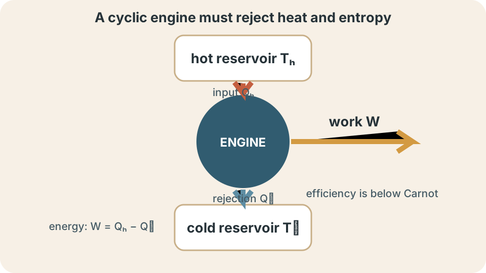
An engine absorbs $Q_h$ from a hot reservoir, produces work $W$, and rejects $Q_c$ to a cold reservoir. The first law gives $W=Q_h-Q_c$ when all quantities denote positive magnitudes. Setting $Q_c=0$ would give one hundred percent conversion. The second law prevents that cyclic limit for finite reservoir temperatures. Entropy rejection requires nonzero $Q_c$.

Clausius and Kelvin–Planck statements are equivalent forms of the second law. Violating one could be combined with an ordinary device to violate the other. Their wording emphasizes different impossible machines. Both express constraints on cyclic energy conversion. Entropy provides a quantitative language for those constraints.

Heat-engine efficiency

Thermal efficiency is desired work output divided by heat input: $\eta=\frac{W}{Q_h}$. Substituting the first law gives $\eta=1-\frac{Q_c}{Q_h}$. Efficiency is dimensionless because numerator and denominator have the same energy unit. It is often reported as a percentage. The symbol $\eta$ is Greek eta.

A real engine has $0<\eta<1$ under ordinary operation. A larger rejected heat $Q_c$ lowers efficiency for fixed $Q_h$. Work does not equal a substance removed from heat. It is an energy transfer mode. The engine returns to its initial state each cycle.

Efficiency alone does not report power. A highly efficient engine operating slowly may deliver little work per second. Power has unit watt, $\mathrm{\frac{J}{s}}$. Efficiency compares energy amounts. Performance analysis may need both quantities.

Carnot’s reversible limit

For a reversible engine between constant-temperature reservoirs, entropy transfers cancel: $\frac{Q_h}{T_h}=\frac{Q_c}{T_c}$. Rearranging gives $\frac{Q_c}{Q_h}=\frac{T_c}{T_h}$. Substitute into the efficiency expression. The maximum is $\eta_{\max}=1-\frac{T_c}{T_h}$. Both temperatures are in kelvins.

The Carnot limit depends only on reservoir temperatures, not working substance. Raising $T_h$ or lowering $T_c$ increases the ideal limit. Reaching absolute zero is impossible, so perfect efficiency is unavailable. Material limits and heat-transfer rates also constrain real devices. Reservoir temperatures bound every engine operating between them.

For $T_h=600\,\mathrm K$ and $T_c=300\,\mathrm K$, $\eta_{\max}=1-\frac{300}{600}=0.500=50.0\%$. A claimed $70.0\%$ engine between these reservoirs violates the second law. A real device must perform below the limit. The bound is a screening tool. Kelvin units cancel in the ratio.

Why real engines fall below Carnot

Real heat transfer occurs across finite temperature differences. Friction converts organized motion into internal energy. Fluids expand through pressure drops. Electrical resistance, mixing, turbulence, and chemical nonequilibrium generate entropy. Each irreversibility reduces available work.

For a cyclic engine, working-fluid entropy returns to its initial value. Generated entropy must be exported with rejected heat. At fixed reservoir temperatures and heat input, more entropy generation generally requires more rejection. First-law relation then leaves less work. The entropy penalty becomes an efficiency penalty.

Carnot operation requires ideal reversible steps and infinitesimal driving differences. Such a device would operate arbitrarily slowly in the strict limit and deliver vanishing power. Practical design balances efficiency, power, size, cost, and durability. Maximum efficiency is not automatically maximum usefulness. Real optimization includes competing objectives.

Reversible and quasistatic are different

A quasistatic process passes through states close to equilibrium. It proceeds slowly enough that state variables remain well defined. This condition can help reversibility. It is not sufficient. Friction can dissipate energy even during slow motion.

A reversible process can be reversed by an infinitesimal change while leaving no net change in system and surroundings. It requires no entropy generation. Heat transfer occurs through infinitesimal temperature differences. Mechanical motion avoids friction and unrestrained expansion. It is an ideal limit.

Rapid processes are usually irreversible, but slowness does not guarantee reversibility. A slowly stirred viscous fluid generates entropy. A slowly leaking gas through a pressure drop generates entropy. Always inspect mechanisms. Do not infer reversibility from time scale alone.

Isothermal ideal-gas expansion

For a reversible isothermal expansion of an ideal gas, internal energy change is zero because ideal-gas internal energy depends only on temperature. The first law then gives heat into the gas equal to work done by the gas. Reversible work is $W=nRT\ln\left(\frac{V_f}{V_i}\right)$. The logarithm’s argument is dimensionless. Final and initial volumes must use matching units.

At constant temperature, gas entropy change is $\Delta S_{\mathrm{gas}}=\frac{Q_{\mathrm{rev}}}{T}=nR\ln\left(\frac{V_f}{V_i}\right)$. If one mole expands from $V_i$ to $2V_i$, then $\Delta S=R\ln2$. Using $R=8.314\,\mathrm{\frac{J}{mol\,K}}$ gives $5.76\,\mathrm{\frac{J}{K}}$. Mole units cancel. The positive sign matches increased accessible volume.

For a reversible path, surroundings lose the same entropy. Universe entropy change is zero. For a free expansion between the same gas states, system entropy change is still $nR\ln2$ because entropy is a state function. No heat need enter, so entropy is generated internally. Same endpoints do not imply same generation.

Free expansion exposes state versus path

Imagine an ideal gas expanding into an evacuated chamber inside an insulated rigid container. Boundary work is zero because no external pressure resists expansion. Heat transfer is zero because the container is insulated. The first law gives $\Delta U=0$. Ideal-gas temperature remains unchanged under the simple model.

Yet volume increases and gas entropy increases by $nR\ln\left(\frac{V_f}{V_i}\right)$. The entropy transfer term is zero. Therefore the entire increase is $S_{\mathrm{gen}}>0$. The process is irreversible. Energy conservation and entropy generation coexist.

To restore the gas and surroundings exactly would require external intervention. Compression would require work and cause changes elsewhere. The spontaneous reverse does not occur. This example cleanly separates stored energy from accessible arrangement. Entropy identifies the lost reversibility.

Statistical interpretation

Boltzmann’s relation is $S=k_B\ln\Omega$ for an idealized macrostate count. Constant $k_B=1.380649\times10^{-23}\,\mathrm{\frac{J}{K}}$ is Boltzmann’s constant. Symbol $\Omega$ counts compatible microstates under the model. The logarithm makes entropy additive for independent multiplicative counts. Greater multiplicity means greater entropy.

A macrostate specifies coarse quantities such as energy, volume, and particle number. A microstate specifies far more detailed microscopic information. Many microstates can correspond to one macrostate. Systems overwhelmingly occupy macrostates with enormous multiplicity because vastly more microscopic arrangements realize them. Probability supports thermodynamic direction.

The word “disorder” can be suggestive but is unreliable. A crystal can have substantial entropy, and visually mixed states are not defined precisely by messiness. Energy dispersal and multiplicity are more disciplined ideas. Calculation requires a model, not an aesthetic judgment. Statistical entropy connects counting to thermodynamic state functions.

Information and thermodynamic entropy

Information entropy and thermodynamic entropy share mathematical structures involving probabilities and logarithms. They are not automatically interchangeable quantities. Thermodynamic entropy carries physical units and relates to energy, temperature, and state. Information entropy depends on a probability model and logarithm base. Context supplies interpretation.

Erasing information in a physical device can have thermodynamic consequences. Landauer’s principle sets a minimum heat cost for logically irreversible bit erasure under ideal conditions. This connection is deep but does not mean every missing fact is heat. A physical implementation and reservoir are required. Careful boundaries prevent loose analogy.

Statistical mechanics derives macroscopic behavior from ensembles of microstates. Probability does not mean thermodynamic laws are casually violated at ordinary scales. Downward total-entropy fluctuations for macroscopic systems are fantastically improbable. Scale explains the apparent certainty. The second law is statistical in origin and extraordinarily reliable in practice.

Entropy rate balances

For processes over time, entropy balance can be written in rate form. A closed-system form is $\frac{dS_{\mathrm{system}}}{dt}=\sum_j\frac{\dot Q_j}{T_j}+\dot S_{\mathrm{gen}}$. A dot denotes rate per unit time. Heat-transfer rate $\dot Q$ has unit watt. Entropy-generation rate has unit $\mathrm{\frac{W}{K}}$.

Steady state does not imply zero entropy generation. It means system entropy content is not changing with time. Entropy entering, leaving, and being generated can balance. A steady heat exchanger is an example. Internal irreversibility persists while macroscopic inlet and outlet conditions remain steady.

Open systems also carry entropy with mass flow. Their balances include terms such as $\dot m s$, where specific entropy $s$ has unit $\mathrm{\frac{J}{kg\,K}}$. Mass flow rate has unit $\mathrm{\frac{kg}{s}}$. The product gives $\mathrm{\frac{W}{K}}$. Boundary choice again determines every term.

Entropy generation and lost work

Entropy generation measures departure from reversibility. Greater generation means less opportunity to convert energy into useful work relative to a chosen environment. The Gouy–Stodola relation connects lost work to ambient temperature times generated entropy under appropriate conditions. This idea is called exergy destruction. It evaluates energy quality.

Energy does not disappear when work potential is lost. It remains conserved, often dispersed as lower-temperature internal energy. The first law sees the quantity. The second law sees reduced usefulness relative to surroundings. Calling this “energy loss” without qualification can be misleading.

Engineering improvement targets large sources of entropy generation. Heat exchangers reduce finite temperature differences within practical size constraints. Bearings reduce friction. Turbomachinery reduces uncontrolled mixing and shocks. Entropy balances identify where work potential is destroyed.

Common misconceptions and repairs

One misconception says entropy always increases everywhere. A subsystem can decrease by exporting entropy. The isolated total cannot decrease. Define system and surroundings. Then add their changes.

Another misconception says entropy is conserved. Energy is conserved, but entropy can be generated. Reversible processes generate zero. Irreversible processes generate positive entropy. A balance must include both transfer and generation.

A third misconception says any slow process is reversible. Friction, resistance, mixing, and finite gradients remain irreversible at low speed. Check mechanisms. A fourth uses Celsius in temperature ratios. Convert every absolute temperature to kelvins.

A reliable entropy-analysis routine

Define the system boundary, initial and final states, and sign convention. Write the first-law energy ledger. Identify every heat interaction and its boundary or reservoir temperature. Calculate system entropy change from state information or a convenient reversible path. Do not insert irreversible heat blindly into the reversible definition.

Write the entropy balance. Include transfer with correct signs. Solve for entropy generation. Verify $S_{\mathrm{gen}}\geq0$. If it is negative, inspect signs, units, temperatures, missing surroundings, and process feasibility.

For cyclic devices, set working-fluid changes over a complete cycle to zero. Use energy conservation and entropy inequality together. Compare efficiency or coefficient of performance with the reversible limit. Report kelvins and appropriate energy units. Explain what creates irreversibility.

Practice and connection forward

Can a system’s entropy decrease? Yes, if it exports enough entropy that total system-plus-surroundings change remains nonnegative. A freezing sample can lose entropy while releasing heat to a warmer environment under an appropriate driven process. The complete ledger decides feasibility. Local decrease does not violate the second law.

Between $900\,\mathrm K$ and $300\,\mathrm K$, Carnot efficiency is $\eta_{\max}=1-\frac{300}{900}=\frac{2}{3}\approx66.7\%$. A real engine must operate below this value. Between $600\,\mathrm K$ and $300\,\mathrm K$, the limit is $50.0\%$. Temperature ratios use kelvins. Efficiency has no physical unit.

Without looking back, explain why energy conservation cannot choose heat-flow direction. Derive the reservoir entropy total and the Carnot limit. Distinguish entropy transfer from generation. Statistical mechanics will connect entropy with microscopic multiplicity. Engineering thermodynamics will use entropy generation to locate lost work potential.