Colligative Properties

Adding a nonvolatile solute to a solvent can lower vapor pressure, raise boiling point, lower freezing point, and produce osmotic pressure. These effects look different macroscopically, yet they share a common origin. Dispersed solute particles change the solvent’s escaping tendency and chemical potential. In an ideal dilute model, the magnitude depends primarily on the number of dissolved particles rather than their chemical identities. Such properties are called colligative, from a word meaning collected together.

The phrase “number of particles” requires care. One mole of glucose ideally remains one mole of dissolved glucose molecules, while one mole of sodium chloride can produce nearly two moles of ions. Real ions interact, associate, and depart from ideal behavior. The van ’t Hoff factor, $i$, accounts for the effective particle count in elementary calculations. It is a model parameter that can be predicted ideally or inferred experimentally.

This lesson will connect particle pictures, phase-equilibrium diagrams, and quantitative equations. Every temperature shift will be treated as a magnitude and then applied with the correct direction. Solvent mass and solution volume will be kept distinct. Worked examples will preserve units through horizontal fraction bars. The aim is to see four manifestations of one thermodynamic idea rather than memorize four unrelated formulas.

Learning objectives and an opening prediction

After this lesson, you should explain why a nonvolatile solute lowers solvent vapor pressure. You should relate that lowering to boiling-point elevation and freezing-point depression. You should calculate temperature shifts using molality and a van ’t Hoff factor. You should interpret osmosis and calculate ideal osmotic pressure. You should also identify volatility, dilution, dissociation, and nonideality as limitations on simple formulas.

Imagine equal molal aqueous solutions of glucose, sodium chloride, and calcium chloride under ideal complete-dissociation assumptions. Predict which has the largest freezing-point depression. Glucose produces one particle per formula unit, sodium chloride produces two, and calcium chloride produces three. Calcium chloride therefore has the largest effective particle molality. Its ideal shift is three times the glucose shift at equal formula-unit molality. This ranking depends on particle count, not on molar mass or whether the solute “feels colder.”

Now ask whether three times the particles always produces exactly three times the effect. At sufficiently low concentration, ideal formulas may approximate that result. At higher concentration, electrostatic interactions cause ions to correlate rather than behave independently. The effective $i$ can be smaller than the ideal integer. Experimental evidence must decide how accurate the ideal comparison is.

The unifying solvent perspective

A pure liquid solvent has a characteristic chemical potential at a given temperature and pressure. Mixing a nonvolatile solute increases the number of possible arrangements and lowers the solvent’s chemical potential in the liquid phase. The pure solvent phases outside the solution do not receive the same mixing contribution. Phase equilibrium therefore occurs at a different temperature or pressure. Vapor pressure, boiling, freezing, and osmosis are different ways of restoring equality of solvent chemical potential.

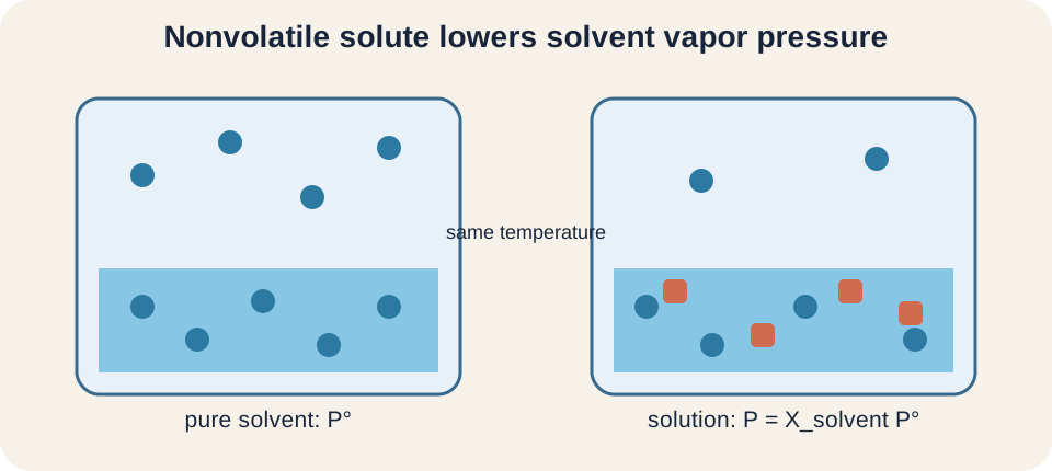
At the particle level, solute particles occupy part of the liquid mixture and reduce the mole fraction of solvent. Fewer solvent molecules are present per unit mixture surface in an idealized picture. That picture helps explain vapor-pressure lowering but should not be mistaken for a complete collision-count mechanism. Interactions and entropy both matter. Chemical potential is the more general thermodynamic quantity connecting them.

Colligative laws work best for dilute solutions because solute particles are then relatively far apart. The solvent behaves nearly like the pure liquid, and activity can be approximated by mole fraction. Solute–solute correlations remain small enough for simple proportionality. As concentration rises, activity coefficients depart from one. The laws become limiting approximations rather than exact identities.

Vapor-pressure lowering and Raoult’s law

For an ideal solution containing a nonvolatile solute, Raoult’s law is $P_{\mathrm{solvent}}=X_{\mathrm{solvent}}P_{\mathrm{solvent}}^{\circ}$. The symbol $P_{\mathrm{solvent}}$ is the solvent partial pressure above the solution. $X_{\mathrm{solvent}}$ is its mole fraction in the liquid, and the superscript circle marks pure-solvent vapor pressure. Mole fraction is dimensionless and lies between zero and one. Therefore the solution solvent pressure is lower than the pure-solvent pressure when solute is present.

The lowering is $\Delta P=P_{\mathrm{solvent}}^{\circ}-P_{\mathrm{solvent}}$. Substitution gives $\Delta P=(1-X_{\mathrm{solvent}})P_{\mathrm{solvent}}^{\circ}$. In a two-component mixture, $1-X_{\mathrm{solvent}}=X_{\mathrm{solute}}$. Thus $\frac{\Delta P}{P_{\mathrm{solvent}}^{\circ}}=X_{\mathrm{solute}}$. The horizontal fraction bar expresses the fractional vapor-pressure lowering.

This form assumes the solute contributes negligible vapor pressure. If both components are volatile, each contributes a partial pressure and total pressure follows Dalton’s law. Strongly nonideal interactions can produce positive or negative deviations from Raoult’s law. A volatile electrolyte or reacting solute needs a more detailed model. Always check the physical identities before applying the nonvolatile-solute formula.

Boiling-point elevation follows vapor pressure

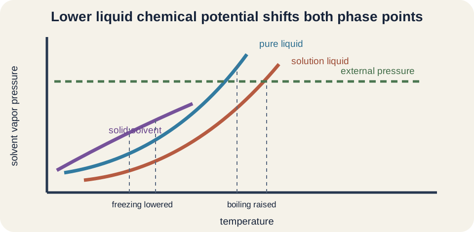
Boiling occurs when a liquid’s vapor pressure equals the external pressure. Because dissolved nonvolatile solute lowers vapor pressure at each temperature, the solution must be heated further to reach the same external pressure. Its boiling point is therefore elevated. The solvent has not acquired a permanently fixed boiling point independent of pressure. Both pure and solution boiling temperatures depend on external pressure.

For dilute solutions, the elevation magnitude is $\Delta T_b=iK_bm$. The symbol $\Delta T_b$ is a positive magnitude in kelvins or Celsius degrees, $i$ is the dimensionless van ’t Hoff factor, $K_b$ is the solvent’s ebullioscopic constant, and $m$ is solute molality. Molality has units $\mathrm{\frac{mol\ solute}{kg\ solvent}}$. Every factor must describe the same solvent and dissolved-particle model. The new boiling temperature is $T_{b,\mathrm{solution}}=T_{b,\mathrm{pure}}+\Delta T_b$.

The constant $K_b$ belongs to the solvent and carries units $\mathrm{\frac{K\,kg}{mol}}$. Multiplying by molality cancels kilograms and moles, leaving kelvins. Celsius temperature differences have the same numerical size as kelvin differences. The formula predicts the shift, not the absolute boiling temperature. Add the positive elevation only after the magnitude is calculated.

Freezing-point depression follows phase balance

Freezing occurs when the solvent has equal chemical potential in liquid solution and solid solvent. The dissolved solute stabilizes the mixed liquid relative to pure solid solvent. A lower temperature is needed before freezing becomes favorable. The solution’s freezing point is therefore depressed. Ideally, the forming solid is nearly pure solvent and excludes the solute.

For a dilute solution, the depression magnitude is $\Delta T_f=iK_fm$. Here $K_f$ is the solvent’s cryoscopic constant with units $\mathrm{\frac{K\,kg}{mol}}$. The new freezing temperature is $T_{f,\mathrm{solution}}=T_{f,\mathrm{pure}}-\Delta T_f$. The formula defines $\Delta T_f$ as a positive magnitude, so subtraction supplies the downward direction. Mixing sign conventions is a common source of double negatives.

Road salt illustrates both usefulness and limits. Dissolved ions lower the equilibrium freezing temperature, helping liquid water persist below $0\,^{\circ}\mathrm C$. Salt does not directly “melt cold” by producing heat in every situation. At sufficiently low temperature, a particular salt–water system reaches a eutectic limit beyond which the simple dilute relation fails. Concentrated brines require phase-diagram data rather than unlimited linear extrapolation.

Molality uses solvent mass

Molality is $m=\frac{n_{\mathrm{solute}}}{m_{\mathrm{solvent}}}$, where the denominator is solvent mass in kilograms. The same letter $m$ is conventionally used for molality, so context and units matter. The numerator is amount of solute in moles. Molality is not moles divided by total solution mass. Labeling the denominator prevents that substitution error.

Molality is useful for temperature-shift equations because mass does not expand appreciably with ordinary temperature changes. Molarity uses liters of solution, and volume changes with temperature. Molality therefore supplies a composition scale independent of container thermal expansion. It also pairs naturally with solvent-specific $K_b$ and $K_f$ units. This convenience does not make molality universally superior for every solution calculation.

Suppose $0.250\,\mathrm{mol}$ glucose dissolves in $500.0\,\mathrm g$ water. Convert solvent mass to $0.5000\,\mathrm{kg}$. Then $m=\frac{0.250\,\mathrm{mol}}{0.5000\,\mathrm{kg}}=0.500\,\mathrm{\frac{mol}{kg}}$. Dividing by $500.0\,\mathrm{kg}$ would be a thousandfold error. Unit conversion should occur before the fraction is evaluated.

The van ’t Hoff factor counts effective particles

The van ’t Hoff factor can be described as $i=\frac{\text{measured colligative effect}}{\text{effect predicted for an equal amount of nonelectrolyte}}$. In an ideal dissociation picture, glucose has $i=1$, sodium chloride has $i=2$, and calcium chloride has $i=3$. These integers follow the numbers of dissolved species in their dissociation equations. They assume complete separation and independent particle behavior. Actual values can differ.

For $\mathrm{CaCl_2(aq)\rightarrow Ca^{2+}(aq)+2Cl^-(aq)}$, one formula unit ideally produces three ions. The coefficient two on chloride counts two chloride particles. Charge does not mean calcium counts twice; each calcium ion is one solute particle for this elementary counting. The ideal factor is therefore three, not four. Stoichiometric coefficients, rather than charge magnitudes, determine ideal count.

Ion pairing and correlated motion reduce the effective number of independent particles. The measured $i$ for an electrolyte often drops as concentration rises. Some molecular solutes associate, while others react or ionize, producing different effective values. A noninteger $i$ is not automatically experimental failure. It can encode real nonideal behavior and chemical equilibria.

Worked example: freezing-point depression

A $0.100\,\mathrm{\frac{mol}{kg}}$ aqueous glucose solution uses $i=1.00$ and water’s $K_f=1.86\,\mathrm{\frac{K\,kg}{mol}}$. The depression magnitude is $\Delta T_f=(1.00)(1.86\,\mathrm{\frac{K\,kg}{mol}})(0.100\,\mathrm{\frac{mol}{kg}})=0.186\,\mathrm K$. Kilograms and moles cancel across the factors. The magnitude has three significant figures. It represents a temperature difference, not the final temperature.

Pure water freezes at approximately $0.000\,^{\circ}\mathrm C$ at standard pressure. Therefore the modeled solution freezing point is $0.000\,^{\circ}\mathrm C-0.186\,^{\circ}\mathrm C=-0.186\,^{\circ}\mathrm C$. The same numerical depression appears in kelvins and Celsius degrees. One should not convert the temperature difference by adding $273.15$. Only absolute temperature values need that offset.

If the same molality were ideal sodium chloride with $i=2.00$, the predicted depression would double to $0.372\,\mathrm K$. A measured value smaller than this could indicate an effective factor below two. Measurement uncertainty, concentration basis, impurities, and supercooling also require consideration. Repeated trials can help separate random variation from systematic departure. The ideal comparison generates a hypothesis rather than proving one mechanism.

Osmosis is selective solvent transport

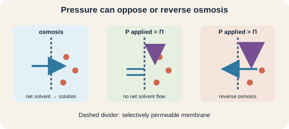
A selectively permeable membrane allows solvent to pass while substantially restricting a solute. If pure solvent lies on one side and solution on the other, net solvent transport tends toward the solution side. This process is osmosis. Solvent moves in both directions microscopically, but the net flow reflects unequal chemical potentials. The process continues until opposing pressure or another contribution restores equilibrium.

Osmotic pressure, $\Pi$, is the extra pressure required on the solution side to stop net osmosis. For an ideal dilute solution, $\Pi=i cRT$. Here $c$ is solute molar concentration in $\mathrm{\frac{mol}{L}}$, $R$ is a gas constant chosen with compatible units, and $T$ is absolute temperature in kelvins. If $R=0.08314\,\mathrm{\frac{L\,bar}{mol\,K}}$, the pressure result is in bar. Celsius cannot replace kelvins in this product.

Osmosis should not be explained as the solute “sucking” water through the membrane. Random molecular motion occurs on both sides. The membrane’s selectivity and the solvent chemical-potential difference create the net transport. Applying sufficient hydrostatic pressure can halt it. Applying still more pressure can reverse the flow, the basis of reverse osmosis.

Worked example: osmotic pressure and molar mass

Suppose $0.0100\,\mathrm{mol}$ of a nonelectrolyte is present in $0.500\,\mathrm L$ solution at $298\,\mathrm K$. Concentration is $c=\frac{0.0100\,\mathrm{mol}}{0.500\,\mathrm L}=0.0200\,\mathrm{\frac{mol}{L}}$. With $i=1.00$ and $R=0.08314\,\mathrm{\frac{L\,bar}{mol\,K}}$, $\Pi=(1.00)(0.0200)(0.08314)(298)=0.496\,\mathrm{bar}$. Liter, mole, and kelvin units cancel. The remaining bar unit is pressure.

Osmotic pressure can estimate molar mass of a large molecule. If sample mass, solution volume, temperature, and $\Pi$ are measured, concentration can be written as $c=\frac{n}{V}=\frac{m_{\mathrm{sample}}}{M V}$. Here $M$ is molar mass, not molarity. Substitution into the osmotic equation allows solving for $M$. This method can be sensitive because even dilute macromolecule solutions produce measurable pressure.

Biological solutions require cautious interpretation. Membranes may pass water and some solutes at different rates, cells actively transport ions, and solutes can dissociate or bind. Tonicity concerns sustained volume effects on cells and is not identical to total osmolarity. A solute that crosses the membrane may contribute transient osmotic pressure but not lasting tonicity. The ideal equation is a foundation, not a complete cell model.

Phase diagrams unify the temperature effects

Plot solvent vapor pressure against temperature for solid, pure liquid, and solution. Adding nonvolatile solute lowers the liquid solvent curve. Its intersection with external pressure moves to a higher temperature, explaining boiling elevation. Its intersection with the solid-solvent curve moves to a lower temperature, explaining freezing depression. Both shifts follow from one altered liquid chemical potential.

This graphical model corrects the idea that solute directly “raises heat” or “adds cold.” The temperature changes arise because phase-equilibrium conditions move. Heating and cooling merely navigate the new phase relationships. The solute need not chemically react with the solvent. Both intersection shifts follow from the altered liquid curve. Particle dispersal changes the thermodynamic state of the liquid mixture.

At higher concentration, curves need not shift linearly with molality. Solids can incorporate solute, multiple solid phases can form, and eutectic behavior can appear. Volatile solutes contribute to vapor composition. Activities replace simple mole fractions. Real phase diagrams then provide the appropriate evidence.

Common misconceptions and repairs

One misconception says colligative properties ignore solute identity completely. Identity matters indirectly through dissociation, association, volatility, interactions, and solubility. The ideal dilute formulas suppress those details into particle number and empirical constants. They do not claim all solutes behave identically at all concentrations. State the model assumptions whenever making the comparison.

Another misconception uses kilograms of solution in molality. The denominator must be kilograms of solvent. A solution made from $10.0\,\mathrm g$ solute and $90.0\,\mathrm g$ water has $0.0900\,\mathrm{kg}$ solvent, not $0.1000\,\mathrm{kg}$. Using total mass systematically underestimates molality. A labeled mass ledger prevents the error.

A third misconception adds freezing depression rather than subtracting it. $\Delta T_f=iK_fm$ is conventionally a positive magnitude. The new freezing temperature is pure-solvent temperature minus that magnitude. Boiling elevation is added. Writing the direction equation before inserting numbers fixes the sign.

Practice with guided feedback

First, rank equal-molality ideal glucose, sodium chloride, and aluminum chloride solutions by freezing depression. Second, explain why molality rather than molarity appears in the temperature-shift formulas. Third, state what pressure must do to stop osmosis. Fourth, identify two reasons a measured electrolyte factor may be noninteger. Explain each response with particles and equations.

Ideal factors are one for glucose, two for sodium chloride, and four for aluminum chloride because $\mathrm{AlCl_3}$ ideally yields one aluminum ion and three chloride ions. Thus aluminum chloride gives the largest modeled depression. Molality uses solvent mass, which is temperature stable, and matches the solvent constants’ units. Opposing pressure on the solution side must equal osmotic pressure to stop net solvent flow. Ion pairing and incomplete dissociation are two possible causes of noninteger $i$.

For a numerical check, use $0.200\,\mathrm{\frac{mol}{kg}}$ nonelectrolyte and $K_b=0.512\,\mathrm{\frac{K\,kg}{mol}}$. The boiling elevation is $\Delta T_b=(1)(0.512)(0.200)=0.102\,\mathrm K$ to three significant figures. If the pure solvent boils at $100.000\,^{\circ}\mathrm C$ under the specified pressure, the modeled solution boils at $100.102\,^{\circ}\mathrm C$. The elevation is added because boiling point moves upward. The result is small because the solution is dilute.

Retrieval and connection forward

Without looking back, name the four colligative effects and connect each to solvent chemical potential. Write $\Delta T_b$, $\Delta T_f$, and $\Pi$ equations and define every symbol with units. Explain why $i$ may be predicted as an integer yet measured as a noninteger. Distinguish solvent mass from solution volume. Finish by describing why boiling rises while freezing falls.

The next thermodynamics lessons make entropy and chemical potential more explicit. Equilibrium lessons replace ideal concentrations with activities when accuracy requires it. Electrolyte theory explains ionic correlations behind deviations in $i$. Biological transport applies osmotic reasoning to membranes with multiple permeabilities. Each extension preserves the central habit of matching a model to its assumptions.

Keep one synthesis statement available. A dissolved nonvolatile solute lowers the solvent’s chemical potential, moving phase-equilibrium conditions and creating a driving force across selective membranes. Ideal dilute effects scale with effective dissolved-particle concentration. Molality supports temperature shifts, while molarity supports the elementary osmotic-pressure equation. Units, particle accounting, and nonideality decide whether a numerical result is trustworthy.