Rate Laws and Reaction Order

Begin with an experimentally determined relationship

A rate law states how reaction rate depends on concentration under specified conditions. For a reaction involving species $A$ and $B$, an empirical form is $r=k[A]^m[B]^n$. The symbol $r$ is normalized reaction rate, $k$ is the rate constant, square brackets denote molar concentration, and exponents $m$ and $n$ are reaction orders. Those exponents must usually be determined from data rather than copied from the balanced equation. The equation summarizes observed dependence but does not by itself prove a molecular mechanism.

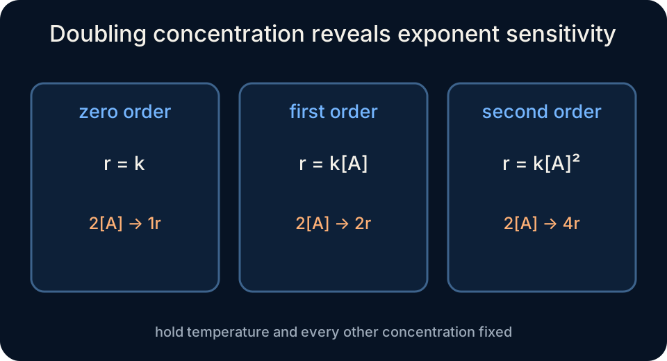
Reaction order tells how sensitively rate responds to a concentration change. If order in $A$ is one, doubling $[A]$ doubles rate while other variables remain fixed. If order is two, doubling $[A]$ multiplies rate by $2^2=4$. If order is zero, changing $[A]$ does not change rate within the measured regime. Noninteger and negative orders are possible in complex mechanisms, so order is not fundamentally a count of molecules.

This lesson develops rate laws through comparison, units, graphs, and time evolution. We will use initial-rate data to determine exponents, calculate $k$, interpret overall order, derive units, distinguish differential from integrated rate laws, and test zero-, first-, and second-order models. We will also connect half-life behavior with order and explain what a fitted law can and cannot reveal about mechanism. Every algebraic step will preserve units and controlled variables. By the end, you should be able to justify a rate law from evidence rather than select one by resemblance.

Read orders as exponents and controls

In $r=k[A]^m[B]^n$, the order with respect to $A$ is $m$ and the order with respect to $B$ is $n$. Overall order is $m+n$ for this multiplicative form. The exponents apply to numerical activities or concentration approximations relative to a standard state, although introductory laws commonly display concentration units directly. Temperature, solvent, catalyst, and ionic environment must remain specified because they can change $k$ or even the observed form. A rate law belongs to a reaction system under conditions, not to a bare balanced equation forever.

To isolate one order, compare experiments in which only that reactant concentration changes. Dividing rate laws cancels $k$ and every unchanged concentration factor. If $[A]$ changes by a factor $f_A$ and rate changes by $f_r$, then $f_r=f_A^m$. Taking logarithms gives $m=\frac{\ln f_r}{\ln f_A}$. The logarithm is useful for changes that are not simple powers of two.

Controlled comparison is essential because changing two concentrations simultaneously mixes their effects. A rate increase cannot then be assigned uniquely to either order without additional equations. Tables should be scanned for experiment pairs differing in one variable. If no such pair exists, simultaneous algebra or regression may estimate several exponents. Experimental design determines how clearly causal sensitivity can be inferred.

Determine orders from initial rates

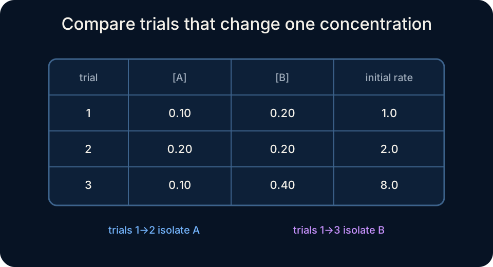
Suppose experiments for $A+B\rightarrow$ products give rates while temperature is constant. Comparing trials one and two, $[A]$ doubles while $[B]$ is unchanged and rate doubles. The ratio equation is $\frac{r_2}{r_1}=\left(\frac{[A]_2}{[A]_1}\right)^m$, so $2=2^m$ and $m=1$. The reaction is first order in $A$. This conclusion depends on the controlled $B$ concentration.

Comparing another pair, $[B]$ triples while $[A]$ is unchanged and rate increases ninefold. The ratio is $9=3^n$, giving $n=2$. The empirical law is therefore $r=k[A][B]^2$. Overall order is $1+2=3$. The balanced coefficients need not match these experimentally determined exponents.

Initial rates are useful because starting concentrations are known and product concentration is minimal. Reverse reaction, inhibition by products, or catalyst change may become more important later. Each rate should be measured over a short interval that still exceeds mixing and instrument dead time. Replicate measurements reveal variability in the inferred ratios. An order should carry uncertainty rather than be forced to the nearest integer without evidence.

Calculate the rate constant and its units

After orders are known, any experiment can determine $k$ through $k=\frac{r}{[A]^m[B]^n}$. Multiple experiments should produce comparable $k$ values if the law and controlled conditions are valid. Large systematic variation signals measurement error, changing conditions, or an unsuitable model. Averaging inconsistent constants can hide rather than solve a model failure. Calculate and compare each value before summarizing.

Units of $k$ depend on overall order because rate always has concentration-per-time units. If overall order is $p$, then $[k]=\frac{\text{concentration}^{1-p}}{\text{time}}$. For first order, $k$ has units $\mathrm{s^{-1}}$. For second order, it has $\frac{\mathrm{L}}{\mathrm{mol\,s}}$, and for zero order it has $\frac{\mathrm{mol}}{\mathrm{L\,s}}$. Units are derived from dimensional balance rather than memorized as unrelated cases.

Suppose $r=2.40\times10^{-4}\,\frac{\mathrm{mol}}{\mathrm{L\,s}}$ when $[A]=0.200\,\frac{\mathrm{mol}}{\mathrm{L}}$ and $[B]=0.100\,\frac{\mathrm{mol}}{\mathrm{L}}$ for $r=k[A][B]^2$. Substitution gives $k=\frac{2.40\times10^{-4}}{(0.200)(0.100)^2}=0.120\,\frac{\mathrm{L^2}}{\mathrm{mol^2\,s}}$. Concentration powers in the denominator produce the units for a third-order law. Recombining $k[A][B]^2$ restores rate units. This dimensional return is a strong algebra check.

Distinguish differential and integrated laws

A differential rate law relates instantaneous rate to current concentration. For a single-reactant disappearance, $-\frac{d[A]}{dt}=k[A]^p$. It answers how fast concentration is changing at a specified moment. An integrated rate law relates concentration directly to elapsed time after solving the differential equation. It answers how much reactant remains at a specified time.

Integration requires an initial condition $[A]_0$ at $t=0$. The resulting form depends on order because the concentration power changes the mathematical accumulation. Zero order gives $[A]_t=[A]_0-kt$. First order gives $\ln[A]_t=\ln[A]_0-kt$. Second order gives $\frac{1}{[A]_t}=\frac{1}{[A]_0}+kt$.

The subscript zero means initial concentration and subscript $t$ means concentration at elapsed time $t$. The natural logarithm $\ln$ is dimensionally applied to an activity ratio, though introductory notation often abbreviates it as $\ln[A]$. Integrated forms assume the same rate law and constant $k$ throughout the interval. Temperature change or mechanism change can invalidate a straight-line test. The fitted interval must therefore be reported with the model.

Test zero-order behavior

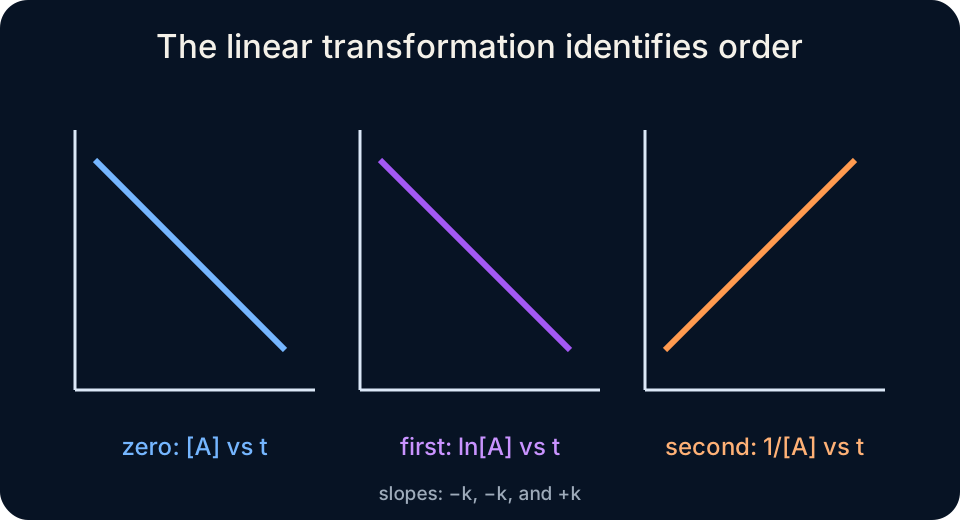
For zero order, rate is $-\frac{d[A]}{dt}=k$ and does not depend on $[A]$ in the observed range. Integration gives $[A]_t=[A]_0-kt$. A plot of $[A]$ against $t$ should be linear with slope $-k$ and intercept $[A]_0$. The negative slope records reactant disappearance. Zero order can occur when a catalyst surface is saturated or light intensity limits a photochemical process.

If $[A]_0=0.500\,\frac{\mathrm{mol}}{\mathrm{L}}$ and $k=0.0200\,\frac{\mathrm{mol}}{\mathrm{L\,s}}$, then after $10.0\,\mathrm{s}$, $[A]_t=0.500-(0.0200)(10.0)=0.300\,\frac{\mathrm{mol}}{\mathrm{L}}$. Units of $kt$ reduce to concentration. The model predicts complete depletion at $25.0\,\mathrm{s}$. It must not be extrapolated past zero concentration because negative concentration is unphysical. A later mechanism or limiting condition must replace the linear law before that point if necessary.

Zero-order half-life depends on initial concentration. Setting $[A]_t=\frac{[A]_0}{2}$ gives $t_{1/2}=\frac{[A]_0}{2k}$. A larger initial amount takes longer to halve at the same constant disappearance rate. Successive halvings become shorter because equal concentration amounts are removed per time. This pattern distinguishes zero order from first-order constant fractional decay.

Test first-order behavior

For first order, $-\frac{d[A]}{dt}=k[A]$. Integration gives $\ln[A]_t=\ln[A]_0-kt$, or equivalently $[A]_t=[A]_0e^{-kt}$. A plot of $\ln[A]$ against time should be linear with slope $-k$. The exponential form shows that equal time intervals remove equal fractions rather than equal concentration amounts. Radioactive decay and many unimolecular processes follow first-order models.

If $k=0.0300\,\mathrm{s^{-1}}$ and $[A]_0=0.800\,\frac{\mathrm{mol}}{\mathrm{L}}$, then after $20.0\,\mathrm{s}$, $[A]_t=(0.800)e^{-(0.0300)(20.0)}=0.439\,\frac{\mathrm{mol}}{\mathrm{L}}$. The exponent is dimensionless because seconds cancel. Concentration remains positive and decreases asymptotically. Substituting the result into the logarithmic form gives the same value. Agreement between equivalent forms is an algebraic consistency check.

First-order half-life is $t_{1/2}=\frac{\ln2}{k}$. It does not depend on initial concentration because exponential decay removes the same fraction each half-life. For $k=0.0300\,\mathrm{s^{-1}}$, $t_{1/2}=23.1\,\mathrm{s}$. Successive halves require equal times. This constant-half-life signature is powerful evidence for first-order behavior.

Test second-order behavior

For the single-reactant law $-\frac{d[A]}{dt}=k[A]^2$, integration gives $\frac{1}{[A]_t}=\frac{1}{[A]_0}+kt$. A plot of reciprocal concentration against time should be linear with slope $k$ and intercept $\frac{1}{[A]_0}$. The positive slope reflects growing reciprocal concentration as reactant decreases. Second-order behavior can arise from a rate-determining encounter between two identical reactant species. Other mechanisms can also produce the same empirical dependence.

If $[A]_0=0.250\,\frac{\mathrm{mol}}{\mathrm{L}}$, $k=0.400\,\frac{\mathrm{L}}{\mathrm{mol\,s}}$, and $t=15.0\,\mathrm{s}$, then $\frac{1}{[A]_t}=4.00\,\frac{\mathrm{L}}{\mathrm{mol}}+6.00\,\frac{\mathrm{L}}{\mathrm{mol}}=10.00\,\frac{\mathrm{L}}{\mathrm{mol}}$. Taking the reciprocal gives $[A]_t=0.100\,\frac{\mathrm{mol}}{\mathrm{L}}$. Units of $kt$ match reciprocal concentration. The result is lower than the initial value and remains positive. Substitution into the differential law predicts a slower rate at this reduced concentration.

Second-order half-life is $t_{1/2}=\frac{1}{k[A]_0}$. It increases as concentration falls, so successive halvings take longer. Doubling initial concentration halves the first half-life. This behavior contrasts with first-order independence and zero-order direct proportionality. Half-life trends provide a model test even when full regression is unavailable.

Evaluate linearized plots carefully

Testing order by linearization means plotting $[A]$, $\ln[A]$, and $\frac{1}{[A]}$ against time and comparing model adequacy. The most linear appearance is not enough because axis transformations change visual spacing and error structure. Residual plots should show random scatter around zero for the selected model. Slope units must agree with the corresponding $k$ units. A mechanistically implausible fit deserves scrutiny even when its correlation is high.

Measurement uncertainty may not remain uniform after transformation. Equal absolute concentration uncertainty becomes asymmetric in reciprocal space and concentration-dependent in logarithmic space. Nonlinear regression of the untransformed integrated model can better reflect original measurement errors. Introductory linear plots remain useful for interpretation and manual analysis. Their limitations should be acknowledged rather than ignored.

Data should span enough concentration change to distinguish curvature. Over a short interval, many smooth curves appear nearly linear in every transformation. Replicate measurements and a broad but valid range strengthen order inference. Late data near detection limits can dominate transformed plots and require appropriate weighting. Model selection combines statistics, measurement quality, and chemical reasoning.

Relate empirical law and mechanism cautiously

For an elementary reaction step, rate-law exponents often match molecularity because the step occurs in one molecular event. For an overall multistep reaction, balanced coefficients generally do not determine observed orders. Intermediates, pre-equilibria, steady states, and the slowest influential steps shape the law. An empirical rate law constrains possible mechanisms but rarely proves one uniquely. Multiple mechanisms can produce the same mathematical dependence.

A species absent from the overall equation can influence rate as a catalyst. Its concentration may appear in a detailed rate law even though it is regenerated and cancels from the net equation. A reactant in the balanced equation can have zero observed order if a surface is saturated. Product inhibition can introduce additional factors. These cases reinforce that a rate law describes pathway dynamics rather than only stoichiometric bookkeeping.

Temperature changes $k$ even when reaction orders remain the same. The Arrhenius relation $k=Ae^{-E_a/(RT)}$ connects rate constant with activation energy and temperature. Comparing concentration effects requires constant temperature so that $k$ remains controlled. A catalyst can change the pathway and therefore the value or form of the rate law. Experimental conditions belong beside every reported kinetic model.

Diagnose common order errors

The first error is copying balanced coefficients into rate exponents without evidence. Only a known elementary step authorizes that direct connection. The second is comparing experiments where several concentrations change and assigning the whole rate effect to one species. The third is calculating $k$ before determining orders. A structured ratio comparison prevents these errors.

Another error is using the wrong integrated plot direction. Zero order linearizes concentration, first order logarithmic concentration, and second order reciprocal concentration. Slope signs also differ: zero- and first-order reactant plots have slope $-k$, while reciprocal second-order plots have slope $+k$. Units can identify a mismatch. A claimed first-order constant with second-order units is internally inconsistent.

Rounding orders too aggressively can hide uncertainty or mixed behavior. An estimated order $1.47$ should not automatically become one or two without examining experimental precision and theory. A changing apparent order may signal competing mechanisms or a limited concentration regime. Report methods and uncertainty with the fitted value. Reaction order is an empirical conclusion, not a decorative integer.

Practice the evidence chain

First, doubling $[A]$ at fixed $[B]$ doubles rate, while doubling $[B]$ at fixed $[A]$ multiplies rate by eight. The first comparison gives $2=2^m$ and $m=1$. The second gives $8=2^n$ and $n=3$. The law is $r=k[A][B]^3$ with overall order four. The exponents come from controlled ratios rather than equation coefficients.

Second, determine which plot tests a first-order model. Plot $\ln[A]$ vertically against time horizontally and look for a linear relationship with random residuals. The slope is $-k$ and has inverse-time units. The intercept is $\ln[A]_0$ in the abbreviated concentration notation. A concentration-versus-time curve itself should show exponential decay rather than a straight line.

Third, compare half-life patterns. Constant half-life supports first order, decreasing successive half-lives support zero order, and increasing successive half-lives support second order for the simple single-reactant cases. The pattern should be evaluated across multiple halvings and above detection limits. Temperature and conditions must remain controlled because $k$ can change. Half-life evidence complements rather than replaces full concentration-time analysis.