Measuring Reaction Rates

Begin with change measured against time

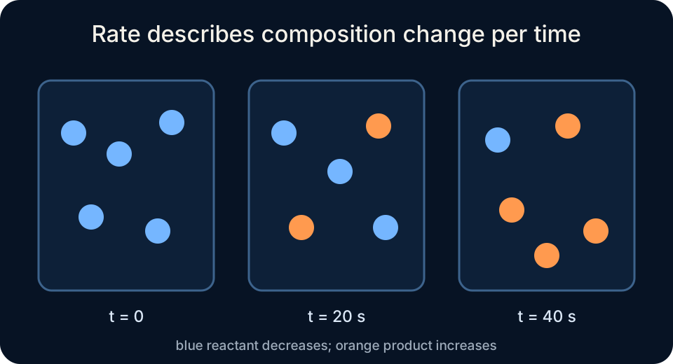
Chemical kinetics studies how rapidly composition changes and which molecular processes control that change. A reaction can be thermodynamically favorable yet proceed slowly because thermodynamics compares states while kinetics describes pathways and rates. Rate is not simply “how much product exists,” because an accumulated amount does not reveal how long formation required. Instead, rate compares a change in a measurable reaction-progress quantity with the elapsed time. The chosen quantity might be concentration, gas pressure, mass, absorbance, conductivity, or another signal calibrated to composition.

For a reactant $A$, an average disappearance rate over a time interval is $-\frac{\Delta[A]}{\Delta t}$. Square brackets mean molar concentration, $\Delta[A]=[A]_f-[A]_i$ is final concentration minus initial concentration, and $\Delta t=t_f-t_i$ is elapsed time. Reactant concentration decreases, making $\Delta[A]$ negative, so the leading minus sign makes disappearance rate positive. If concentration is measured in $\frac{\mathrm{mol}}{\mathrm{L}}$ and time in seconds, rate has units $\frac{\mathrm{mol}}{\mathrm{L\,s}}$. Units and sign together communicate what quantity changes and in which direction.

This lesson connects operational measurement with reaction equations and graphs. We will define average and instantaneous rates, normalize different species rates with coefficients, interpret concentration–time slopes, select observable signals, design sampling intervals, and analyze uncertainty. Each formula will be related to the graph or apparatus from which its numbers arise. Examples will report units throughout and distinguish raw signal from chemical concentration. By the end, you should be able to plan a defensible rate measurement and explain what the resulting number means physically.

Define average rate over a finite interval

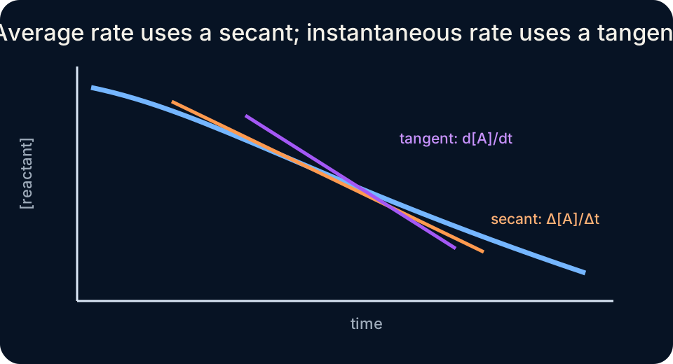
Average rate describes a secant slope between two measured states. If reactant concentration falls from $0.800\,\frac{\mathrm{mol}}{\mathrm{L}}$ at $10.0\,\mathrm{s}$ to $0.620\,\frac{\mathrm{mol}}{\mathrm{L}}$ at $40.0\,\mathrm{s}$, then $\Delta[A]=-0.180\,\frac{\mathrm{mol}}{\mathrm{L}}$. The elapsed time is $30.0\,\mathrm{s}$. Disappearance rate is $-\frac{-0.180\,\frac{\mathrm{mol}}{\mathrm{L}}}{30.0\,\mathrm{s}}=6.00\times10^{-3}\,\frac{\mathrm{mol}}{\mathrm{L\,s}}$. The result averages all rate variation within that thirty-second interval.

For a product $P$, concentration increases and average appearance rate is $+\frac{\Delta[P]}{\Delta t}$. A leading negative sign is unnecessary because $\Delta[P]$ is normally positive while product accumulates. Rate signs are conventions chosen to report forward progress positively, not evidence that concentration changes lost their algebraic sign. A full statement names appearance or disappearance and the species involved. Without those labels, two equal positive numbers could represent different physical observations.

Average rate depends on interval length and location when a reaction slows or accelerates. A long interval smooths fluctuations but can hide rapid early change, while a short interval provides local detail but magnifies measurement noise. Comparing rates requires intervals and definitions to be stated. A secant line on a concentration–time graph visualizes the chosen interval and slope. Reporting only endpoints without the interval conceals the temporal resolution of the result.

Connect species rates through stoichiometry

Different species concentrations change at different numerical rates when their coefficients differ. For $aA+bB\rightarrow cC+dD$, a single reaction rate is defined as $r=-\frac{1}{a}\frac{d[A]}{dt}=-\frac{1}{b}\frac{d[B]}{dt}=\frac{1}{c}\frac{d[C]}{dt}=\frac{1}{d}\frac{d[D]}{dt}$. Lowercase coefficients $a$, $b$, $c$, and $d$ come from the balanced equation. The derivative notation $\frac{d[A]}{dt}$ means instantaneous concentration slope with respect to time. Dividing by coefficients removes species-dependent scaling.

For $\mathrm{2N_2O_5\rightarrow4NO_2+O_2}$, nitrogen dioxide appears four times as fast as reaction extent progresses, while oxygen appears once. If oxygen appears at $1.20\times10^{-3}\,\frac{\mathrm{mol}}{\mathrm{L\,s}}$, nitrogen dioxide appears at $4.80\times10^{-3}\,\frac{\mathrm{mol}}{\mathrm{L\,s}}$. Dinitrogen pentoxide disappears at $2.40\times10^{-3}\,\frac{\mathrm{mol}}{\mathrm{L\,s}}$. Dividing each species rate by its coefficient gives the same normalized reaction rate $1.20\times10^{-3}\,\frac{\mathrm{mol}}{\mathrm{L\,s}}$. The shared result confirms that every species follows one balanced reaction progress.

Coefficient normalization is not an optional formatting preference. Without it, asking for “the reaction rate” would yield several numerical answers depending on which species was monitored. The balanced equation synchronizes species changes through reaction extent. A coefficient belongs in the rate definition because composition changes in those fixed ratios. Subscripts inside chemical formulas do not replace equation coefficients and must not be used for normalization.

Interpret instantaneous rate as a tangent slope

Instantaneous rate describes behavior at a particular time rather than across a finite interval. Mathematically, it is the limit of average rate as the interval shrinks, $\frac{d[A]}{dt}=\lim_{\Delta t\to0}\frac{\Delta[A]}{\Delta t}$. The derivative symbol $d$ indicates an infinitesimal change in the limiting definition. On a concentration–time graph, the derivative is the slope of the tangent line at the chosen point. Reactant tangents usually slope downward, while product tangents slope upward.

Experimental data are discrete, so a true infinitesimal interval is not measured directly. A centered finite difference can estimate slope near time $t_i$ using points on both sides: $\frac{[A]_{i+1}-[A]_{i-1}}{t_{i+1}-t_{i-1}}$. The subscripts label neighboring data points rather than chemical coefficients. Smaller spacing can improve temporal locality but increases sensitivity to noise. Curve fitting can use all data to estimate a smooth derivative when an appropriate model is justified.

Initial rate is the instantaneous rate near $t=0$. It is valuable because starting concentrations are known most clearly and product buildup, reverse reaction, or catalyst deactivation may be minimal. Measuring too slowly can miss the initial region, especially for rapid reactions. Mixing time and sensor response impose a practical lower limit on the earliest trustworthy measurement. “Initial” should therefore be defined operationally rather than assumed to mean an inaccessible exact instant.

Choose an observable that tracks composition

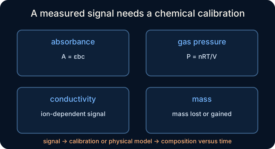
Direct concentration measurement is not always possible during a reaction, so kinetics often uses a calibrated proxy. Spectrophotometry measures absorbance when a reactant or product absorbs light, and Beer’s law $A=\varepsilon bc$ connects absorbance $A$ with concentration $c$. The symbol $\varepsilon$ is molar absorptivity and $b$ is optical path length. A calibration or known absorptivity is required before an absorbance change becomes a concentration change. Absorbance itself is dimensionless, so it cannot be reported as molarity without that relationship.

Gas-forming reactions can be followed through volume or pressure. At controlled temperature and volume, ideal-gas pressure is proportional to gas amount through $P=\frac{nRT}{V}$. At controlled temperature and pressure, collected gas volume is proportional to amount. Temperature, water-vapor pressure, leaks, and gas solubility can affect the signal. The apparatus conditions determine which conversion from signal to moles is valid.

Other methods track mass loss, conductivity, pH, titrated aliquots, or color intensity. Conductivity responds to ion identities and mobilities rather than merely total concentration, so calibration may be nonlinear. Quenching sampled aliquots stops or slows the reaction before later analysis, but the quench itself must act rapidly relative to reaction time. Every method has a response time, range, selectivity, and disturbance risk. Choosing a signal means showing that it changes predictably with the target species while other factors remain controlled.

Design time sampling deliberately

Sampling intervals should be shorter where concentration changes rapidly and may be longer after the reaction slows. Uniform intervals simplify analysis but can waste measurements late and undersample early behavior. Automated sensors can collect frequent data, although more points do not automatically improve accuracy if response time or noise dominates. Manual sampling requires enough time for withdrawal, quenching, and analysis. A pilot experiment helps match the schedule to the reaction timescale.

The measurement should begin from a reproducible time origin. Mixing often defines $t=0$, but manual mixing takes finite time and can create concentration gradients. A stopped-flow apparatus mixes rapidly and observes fast reactions with a known dead time. Slower classroom experiments may define zero when the final reagent is added and use consistent stirring. The method must state how the clock and reaction were synchronized.

Temperature control is critical because rate constants commonly change strongly with temperature. A water bath can equilibrate reagents before mixing and maintain the reaction vessel near a target temperature. Sensor heat, room drafts, or an exothermic reaction can still change sample temperature. Recording temperature alongside concentration data allows deviations to be identified. Comparing trials at different concentrations is meaningful only when other influential variables are controlled.

Separate rate from amount and completion

A fast reaction can produce a small total amount if little reactant is present. A slow reaction can eventually produce a large amount if given sufficient time and material. Rate has amount-per-volume-per-time dimensions in concentration form, while extent or yield has amount dimensions. Completion describes how close composition comes to a limiting or equilibrium state. These concepts answer different questions and should not be collapsed into “more reaction.” Careful vocabulary prevents speed, scale, and final composition from being confused.

The steepness of a graph indicates rate, while the vertical concentration change indicates accumulated composition change. Two curves can reach the same final product concentration with different initial slopes. Conversely, curves can have the same initial slope but different final extents because their starting amounts or equilibria differ. Graph axes and intervals make those distinctions visible. Reading only the endpoint misses the kinetic history.

Equilibrium reactions have equal forward and reverse rates at equilibrium, not zero molecular activity. Concentrations become macroscopically constant because opposing changes cancel. A measured net rate approaches zero while dynamic reaction continues in both directions. Rate-law analysis can distinguish forward and reverse contributions in more advanced models. The plateau of a concentration curve should therefore be interpreted with equilibrium and detection limits in mind.

Process data without hiding uncertainty

Raw data should retain time, measured signal, calibration conversion, units, and uncertainty. Plotting concentration against time reveals outliers, curvature, and possible delay before a rate is calculated. A table of slopes alone hides the shape that justified each estimate. Replicate trials show reproducibility and can reveal whether variation is larger than instrument resolution. Data exclusion requires a documented reason rather than a desire for a smoother graph.

Uncertainty in two concentration measurements propagates into $\Delta[A]$, and timing uncertainty propagates into $\Delta t$. When the concentration difference is small, fixed measurement uncertainty can dominate the calculated slope. Longer intervals increase the difference but reduce local time resolution. This tradeoff explains why a numerically stable average rate may not approximate an instantaneous rate closely. Error bars and sensitivity to interval choice make the limitation visible.

Linear regression can estimate a slope when the selected interval is adequately linear. The slope unit comes from vertical-axis units divided by horizontal-axis units. Residuals should scatter without systematic curvature if a straight-line model is suitable. A high coefficient of determination alone does not prove the kinetic model is correct. Graphical diagnostics and chemical assumptions must support the fitted relationship.

Diagnose common rate errors

The first error is omitting the negative sign for reactant disappearance and then reporting a negative “rate” without explanation. Concentration change may be negative, but the conventional disappearance rate is positive. The second error is forgetting coefficient normalization when comparing species. The third is reporting concentration as a rate without dividing by elapsed time. Units expose all three mistakes.

Another error is drawing a tangent by using a single point. A slope requires change between at least two coordinates or a fitted local model. Using a very wide interval gives an average that may not represent the stated time. Using an extremely narrow noisy interval can produce an unstable estimate. The graphical line and chosen points should be shown or described.

A final error is assuming every changing signal is directly proportional to concentration. Absorbance may follow Beer’s law only within a calibrated range, gas pressure requires controlled volume and temperature, and conductivity depends on several ions. Instrument response can lag behind rapid chemistry. A valid method includes a calibration or physical equation connecting signal with species amount. Measurement design is part of kinetics, not a separate technical afterthought.

Practice a complete rate argument

First, a reactant falls from $0.500\,\frac{\mathrm{mol}}{\mathrm{L}}$ at $20.0\,\mathrm{s}$ to $0.380\,\frac{\mathrm{mol}}{\mathrm{L}}$ at $50.0\,\mathrm{s}$. Its average disappearance rate is $-\frac{0.380-0.500}{50.0-20.0}=4.00\times10^{-3}\,\frac{\mathrm{mol}}{\mathrm{L\,s}}$. The numerator is negative, the leading minus sign makes the rate positive, and the denominator is $30.0\,\mathrm{s}$. This value averages the entire interval. It does not specify the instantaneous rate at either endpoint.

Second, for $\mathrm{2A\rightarrow3B}$, suppose $B$ appears at $0.090\,\frac{\mathrm{mol}}{\mathrm{L\,s}}$. The normalized reaction rate is $r=\frac{1}{3}\frac{d[B]}{dt}=0.030\,\frac{\mathrm{mol}}{\mathrm{L\,s}}$. Reactant $A$ disappears at $2r=0.060\,\frac{\mathrm{mol}}{\mathrm{L\,s}}$. The species rates differ because the coefficients differ. Dividing by coefficients recovers one common reaction-progress rate.

Third, evaluate a plan to measure a rapid colored reaction by reading absorbance manually once per minute. The sampling interval may miss the early change, and manual timing may be slow relative to the reaction. An automated spectrometer with subsecond acquisition and known mixing dead time would better resolve the initial slope. A Beer’s-law calibration must still connect absorbance with concentration and confirm the working range. The improved plan controls temporal resolution, synchronization, and signal interpretation rather than merely collecting more digits.