Dynamic Equilibrium

A sealed reaction mixture can appear unchanged even while molecules continue transforming. The forward reaction converts reactants into products, and the reverse reaction converts products back into reactants. When those two rates become equal, the macroscopic composition remains constant because every interval produces and consumes equal amounts of each participating species. This state is called dynamic equilibrium. The word “dynamic” matters because equilibrium is ongoing balance, not molecular inactivity.

You will learn to distinguish equal rates from equal concentrations, interpret rate-time and concentration-time graphs, explain why a suitable closed system is needed, and trace approach to equilibrium from either direction. You will connect collision-level events with stable bulk measurements. You will also distinguish a temporary disturbance, a shift in composition, and a change in the equilibrium constant. Symbols for concentration, rate, time, and reversible reaction arrows will be explained as they appear. The goal is to build the conceptual foundation needed before calculating equilibrium constants.

Begin every equilibrium argument by identifying the reversible reaction, system boundary, temperature, and variables being observed. Ask whether matter can escape and whether both forward and reverse processes are physically possible. Separate statements about rate from statements about amount or concentration. Describe what changes during the approach and what becomes constant at equilibrium. Finally, avoid using “stops,” “equal concentrations,” or “complete reaction” unless evidence specifically supports those claims.

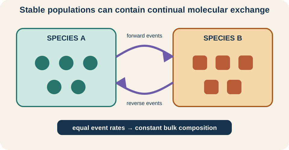
Reversible reactions proceed in both directions

A reversible reaction is represented with opposing arrows, as in $\mathrm{A\rightleftharpoons B}$. The rightward arrow represents conversion of A to B, while the leftward arrow represents conversion of B to A. The symbols A and B are placeholders for chemical species, not necessarily individual atoms. Both directions may occur through one or several molecular steps. The relative rates depend on composition, temperature, catalysts, and the reaction mechanism.

At the start of a mixture containing only A, the forward process can occur while the reverse process initially has no B available. As B forms, reverse events become possible. Simultaneously, depletion of A may reduce the forward rate. The two rates can therefore move toward one another over time. Their equality defines the equilibrium condition.

Some equations are written with a single arrow because the reverse process is negligible under the stated conditions or because the model focuses on one direction. That notation does not mean microscopic reversibility is abolished as a general physical principle. It means the chosen conditions and scale make one direction dominant for practical purposes. Equilibrium analysis is appropriate when both directions contribute appreciably before reactants are exhausted or removed. The arrow notation should follow the model being used.

Equilibrium requires equal forward and reverse rates

Let $r_{\mathrm f}$ denote the forward rate and $r_{\mathrm r}$ denote the reverse rate. Dynamic equilibrium requires $r_{\mathrm f}=r_{\mathrm r}$. A reaction rate measures change in amount or concentration per unit time, so common units include $\frac{\mathrm{mol}}{\mathrm{L\,s}}$. Equality means the two directions produce opposing composition changes of equal magnitude. The net rate is therefore zero.

The net rate can be written $r_{\mathrm{net}}=r_{\mathrm f}-r_{\mathrm r}$ for a simple sign convention. Before equilibrium, a positive net rate indicates net forward progress, while a negative value indicates net reverse progress. At equilibrium, subtraction gives zero even though both individual rates can be nonzero. This is analogous to equal flows into and out of a container maintaining a constant level. Zero net change does not require zero microscopic traffic.

The rate equality applies consistently to balanced stoichiometry. For $\mathrm{N_2O_4\rightleftharpoons2NO_2}$, one forward event consumes one dinitrogen tetroxide unit and produces two nitrogen dioxide units. Rate definitions divide concentration changes by stoichiometric coefficients so a single reaction rate can describe all species. The reverse direction follows the opposite change. Equal reaction rates make every bulk concentration constant together.

Equal rates do not imply equal concentrations

At equilibrium, reactant and product concentrations are constant but generally not equal. For $\mathrm{A\rightleftharpoons B}$, a particular temperature might favor mostly B, mostly A, or comparable amounts. The equality condition concerns rates, which depend on both concentrations and kinetic relationships. Different forward and reverse rate constants can yield equal rates at unequal concentrations. Saying “equilibrium means equal amounts” confuses a special numerical possibility with the definition.

For a simple elementary model, suppose $r_{\mathrm f}=k_{mathrm f}[\mathrm A]$ and $r_{\mathrm r}=k_{mathrm r}[\mathrm B]$. The brackets $[\mathrm A]$ and $[\mathrm B]$ denote molar concentrations, while $k_{mathrm f}$ and $k_{mathrm r}$ are rate constants. At equilibrium, $k_{mathrm f}[\mathrm A]_{\mathrm{eq}}=k_{mathrm r}[\mathrm B]_{\mathrm{eq}}$. Rearranging gives $\frac{[\mathrm B]_{\mathrm{eq}}}{[\mathrm A]_{\mathrm{eq}}}=\frac{k_{mathrm f}}{k_{mathrm r}}$ for this model. Equal concentrations occur only if the rate constants are also equal.

The subscript “eq” identifies an equilibrium value rather than a new species. Constant concentration means repeated measurements give the same bulk value within experimental resolution. Individual A and B molecules do not acquire permanent labels saying they are equilibrium molecules. They can continue interconverting while population totals stay stable. This microscopic turnover is why isotopic tracer experiments can reveal activity inside an apparently unchanged mixture.

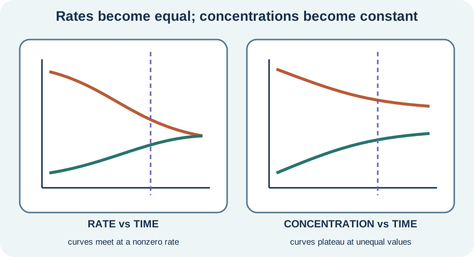
Rate-time graphs show convergence of opposing processes

Imagine starting with mostly reactants. The forward rate is initially high because reactant availability is high, while the reverse rate is low because little product is present. As products accumulate, the reverse rate rises. As reactants are consumed, the forward rate often falls. The curves meet at the equilibrium time and then remain equal under unchanged conditions.

Starting with mostly products reverses the initial pattern. The reverse rate begins high, the forward rate begins low, and net change proceeds toward reactants. The two rate curves still converge at the same equilibrium rate when temperature, total composition, volume, and other constraints match. This approach from either side is strong evidence that equilibrium is a state rather than a memory of preparation history. The path differs while the endpoint relation agrees.

A catalyst changes the shapes and timescales of both curves. It lowers activation barriers for forward and reverse processes, increasing both rates. The curves meet sooner, but the equilibrium composition remains unchanged at fixed temperature because the catalyst does not change the relative thermodynamic stability of states. A rate graph therefore reaches its equality point earlier. The height of the common rate at equilibrium may be larger even though the equilibrium amounts are the same.

Concentration-time graphs level at stable values

A concentration-time graph starting with reactants often shows reactant concentration decreasing and product concentration increasing. The curves flatten when net composition change ceases. Their plateau values need not meet, intersect, or have the same height. Each flat trace indicates a constant concentration. The balanced equation constrains how the changes relate before the plateau.

For $\mathrm{A\rightleftharpoons B}$ with one-to-one stoichiometry in a fixed volume, a decrease $x$ in $[\mathrm A]$ produces an increase $x$ in $[\mathrm B]$. For $\mathrm{A\rightleftharpoons2B}$, a decrease $x$ in A produces an increase $2x$ in B. The variable $x$ represents an extent expressed in concentration units for this simplified bookkeeping. Stoichiometry controls changes, while equilibrium thermodynamics controls the final ratio. Both are needed to interpret a graph quantitatively.

If a disturbance occurs after equilibrium, the concentration graph may show an instantaneous jump for directly altered species followed by a gradual adjustment. A sudden volume decrease changes gas concentrations immediately before chemical reaction has time to respond. Subsequent curved changes reflect the forward and reverse rate imbalance. Distinguishing the vertical jump from the relaxation helps identify what was physically changed. A new plateau represents a new equilibrium composition under the final conditions.

A suitable boundary allows both directions to persist

Equilibrium requires that relevant species remain available for reverse as well as forward reaction. If a gaseous product escapes from an open vessel, its concentration may remain too low for substantial reverse reaction. The system can continue changing rather than settling into the same equilibrium expected in a sealed container. A closed material boundary is therefore common in equilibrium models. Energy may still cross that boundary if temperature is controlled by surroundings.

“Closed” does not mean perfectly isolated. A closed system does not exchange matter with surroundings, while an isolated system exchanges neither matter nor energy in the ideal definition. Many laboratory equilibria are maintained in closed containers immersed in temperature-controlled baths. Heat can flow to establish and hold the specified temperature. The distinction matters because equilibrium constants depend on temperature.

Some open systems maintain steady concentrations through continuous inflow and outflow. That condition may be a steady state rather than thermodynamic equilibrium. Rates of processes can balance macroscopically because material is supplied and removed, even when chemical affinities remain. Biological cells frequently operate in such driven nonequilibrium steady states. Constant concentration alone is therefore insufficient to prove equilibrium.

Microscopic exchange can be observed indirectly

At equilibrium, adding a small amount of isotopically labeled species can reveal ongoing exchange. The label may redistribute among chemical forms even when total concentrations remain constant. Such redistribution would be impossible if reactions had stopped. The bulk equilibrium state hides molecular identity turnover. Tracer evidence makes the dynamic character experimentally accessible.

Evaporation and condensation in a sealed container provide a physical analogue. At vapor–liquid equilibrium, molecules leave the liquid surface while vapor molecules enter it. Equal rates keep the amounts of liquid and vapor statistically constant. Individual molecules can change phase repeatedly. The interface remains active even though the liquid level appears stable.

Saturated dissolution offers another example. In a solution contacting excess solid, ions leave the crystal while dissolved ions rejoin it. At equilibrium, dissolution and crystallization rates match. A marked crystal surface can exchange material without net mass change. The macroscopic observation of constant mass is compatible with continual microscopic events.

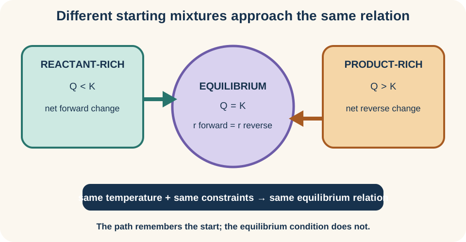
Approach from either side is governed by the reaction quotient

The reaction quotient $Q$ evaluates the current composition using the same activity expression later used for the equilibrium constant $K$. If $Q<K$, the composition is relatively product-poor and net forward change is thermodynamically favored. If $Q>K$, it is relatively product-rich and net reverse change is favored. If $Q=K$, the mixture is at equilibrium. This comparison formalizes the phrase “approach from either side.” The inequalities compare numerical composition ratios for one consistently written reaction.

For $\mathrm{A\rightleftharpoons B}$, a simple idealized quotient is $Q=\frac{a_{\mathrm B}}{a_{\mathrm A}}$, where $a_i$ denotes dimensionless activity. Starting with only A makes $Q$ very small, so net forward change occurs. Starting with mostly B makes $Q$ large, so net reverse change occurs. Both directions move $Q$ toward $K$ under fixed temperature. The endpoint is determined by the constant and conservation constraints.

The quotient predicts net direction, not rate magnitude. A large difference between $Q$ and $K$ can supply a strong thermodynamic driving tendency, yet a high activation barrier may make adjustment slow. A catalyst can accelerate adjustment without changing the target $K$. Thermodynamics and kinetics cooperate in real behavior but answer different questions. Dynamic equilibrium sits at their intersection: thermodynamics sets the composition relation, and kinetics establishes equal opposing rates.

Disturbances create temporary rate inequality

Suppose a system is at equilibrium and more reactant is suddenly added. The forward rate responds immediately because its reactant-dependent collision opportunities increase. The reverse rate initially retains its old value because product concentration has not yet changed. Net forward reaction then consumes some added reactant and produces product. Rates become equal again at a new composition.

This response is often described as an equilibrium shift, but the mechanism is rate imbalance. The disturbance changes one or both instantaneous rates. Reaction changes composition until the opposing rates regain equality. The final composition is constrained by the same $K$ if temperature did not change. Thinking through rates explains the direction instead of relying only on a memorized Le Châtelier slogan.

Changing temperature is different because it changes rate constants unequally and changes the equilibrium constant. The new equilibrium relation may favor a different composition ratio. Changing concentration or volume at fixed temperature changes $Q$ but not $K$ under the model. A catalyst changes both kinetic pathways but changes neither $Q$ instantaneously nor $K$. Classifying the disturbance prevents these effects from being blended.

Temperature determines the equilibrium relation

The equilibrium constant has a fixed value only for a specified temperature and written reaction. Temperature changes molecular energy distributions and the relationship between forward and reverse tendencies. For an endothermic forward reaction, increasing temperature often shifts equilibrium toward products and increases the forward reaction’s $K$ over a relevant range. For an exothermic forward reaction, increasing temperature often shifts toward reactants. These statements can be connected quantitatively through thermodynamics.

Even when temperature changes, the new equilibrium still satisfies equal forward and reverse rates. Their common value and the equilibrium concentrations may all differ from the original state. Rate constants usually increase with temperature for both directions, but not necessarily by identical factors. The ratio associated with equilibrium therefore changes. Faster molecular motion alone does not tell the shift direction.

Temperature must be uniform enough for a single equilibrium description. A system with persistent temperature gradients may exhibit heat flow and local states rather than one global equilibrium. Measurements should be made after thermal and chemical relaxation. Reporting a constant without temperature omits essential information. A numerical equilibrium value is not universal across all conditions.

Catalysts alter approach but not position

A catalyst provides an alternative mechanism with lower activation barriers. It participates in intermediate steps and is regenerated in the overall process. Microscopic reversibility means the catalyzed pathway assists both directions. Therefore the forward and reverse rates increase relative to the uncatalyzed case. Equal-rate equilibrium is reached more quickly.

The catalyst does not change initial or final state energies, standard Gibbs energy, or equilibrium constant at fixed temperature. It cannot make an equilibrium mixture contain more product after full relaxation merely by being present. If an industrial process appears to gain yield with a catalyst, the improvement may arise from reaching equilibrium sooner, suppressing side reactions, or enabling different operating conditions. The direct equilibrium position for the same reaction and conditions remains unchanged. Mechanism and thermodynamic endpoint must be separated.

Removing a catalyst after equilibrium lowers both opposing rates but does not necessarily disturb composition immediately. The system can remain at the same equilibrium composition while exchanging more slowly. If a disturbance follows, relaxation will take longer. This thought experiment reinforces that equilibrium position and equilibrium traffic rate are distinct. Both can be measured, but they are not the same variable.

Equilibrium differs from completion and static balance

A reaction that goes essentially to completion has product-favored equilibrium under the conditions, but the phrase emphasizes that remaining reactant is negligible for the purpose at hand. Dynamic equilibrium remains the underlying limiting concept when reverse reaction is possible. A large equilibrium constant can make the mixture look complete without being mathematically absolute. Experimental detection limits influence the language used. “Complete” is an approximation, not a separate conservation law.

Static balance involves no opposing microscopic processes, while dynamic equilibrium involves equal nonzero processes. A sealed container holding an inert solid at rest is static but not necessarily an example of chemical equilibrium. A balanced object on a table has equal forces, but that mechanical analogy should not be stretched into reaction-rate details. The useful common feature is zero net macroscopic change. The microscopic cause differs by system.

A steady state also differs from equilibrium. Continuous reactant feed and product removal can maintain constant concentrations while net chemical conversion and energy dissipation continue. Forward and reverse reaction rates need not be equal. The system depends on external driving and flux. Constant macroscopic values must therefore be interpreted alongside boundaries and flows.

Common misconceptions and corrective habits

The most common misconception states that reactant and product concentrations are equal at equilibrium. Replace it with the precise condition $r_{\mathrm f}=r_{\mathrm r}$. Concentrations are constant but can differ greatly. Another misconception says reactions stop. Use microscopic exchange or tracer evidence to explain continuing motion.

A second misconception says a catalyst shifts equilibrium toward products. A catalyst accelerates both directions and reduces time to equilibrium without changing $K$ at fixed temperature. A third misconception assumes any flat concentration graph proves equilibrium. Check whether the system is closed and undriven or instead held in a steady state by external flows. Boundary information is part of the diagnosis.

Graph-reading errors often confuse rate curves with concentration curves. Rate curves meet at equilibrium, while concentration curves usually level at different values. Label vertical axes before interpreting intersections or plateaus. A sudden concentration jump may represent the direct disturbance, not instantaneous reaction. Trace the physical sequence from intervention to rate imbalance to relaxation.

Guided practice and retrieval

Suppose only A is initially present for $\mathrm{A\rightleftharpoons B}$. Describe the forward and reverse rates at the first instant and later during approach. The forward rate begins relatively large, while the reverse rate begins at zero if no B exists. As A decreases and B increases, the forward rate tends to fall and the reverse rate tends to rise. Equilibrium begins when the two rates are equal and nonzero. The final concentrations need not be equal.

Now imagine the same equilibrium mixture receives an instantaneous addition of B at constant temperature and volume. The reverse rate responds immediately because B availability increases. Net reverse conversion consumes some B and forms A. The reaction quotient initially becomes larger than the equilibrium constant and then returns toward it. The value of $K$ remains unchanged because temperature is fixed.

Finally compare adding a catalyst with raising temperature. The catalyst shortens relaxation time but does not change the final equilibrium composition under otherwise identical conditions. A temperature change alters the kinetic rates and generally changes the equilibrium constant. Both systems eventually regain equal forward and reverse rates. Only the temperature change establishes a different thermodynamic equilibrium relation.

Connection forward

Reconstruct dynamic equilibrium in one complete explanation. Name the reversible processes, show how their rates change during approach, state the equality condition, and describe why concentrations become constant without becoming necessarily equal. Include the role of a closed boundary and temperature. Then distinguish disturbance, shift, and constant change. If “equilibrium” still sounds like stopping, return to the particle exchange picture.

The equilibrium-constant lesson will quantify the stable composition relationship using dimensionless activities. Reaction quotients will predict the net direction of disturbed mixtures, and ICE tables will connect stoichiometric changes to equilibrium amounts. Acid–base, solubility, and gas equilibria will apply the same framework to specific chemical systems. Kinetics will continue to govern relaxation time. Thermodynamics will explain why the target relation has its temperature dependence.

The enduring insight is balanced traffic. Forward and reverse molecular changes can be individually active while their macroscopic effects cancel. Equal rates create stable composition, but neither equal concentration nor molecular stillness is required. Boundaries determine whether both directions remain available, and temperature determines the equilibrium relation. Once these distinctions are secure, equilibrium calculations become expressions of a physical model rather than symbol manipulation.