Units, Uncertainty, and Significant Figures

A measurement is not merely a number. It is a numerical estimate paired with a unit, a defined quantity, and information about uncertainty. Writing $9.8$ without context leaves the reader unable to decide whether it means metres, seconds, grams, or something else. Writing $9.8\,\mathrm{\frac{m}{s^2}}$ identifies an acceleration. Reporting how that value was obtained and how uncertain it is turns notation into scientific evidence.

Significant figures are one convention for preventing calculated results from implying unsupported precision. They are not a substitute for uncertainty analysis, instrument knowledge, or statistical reasoning. Their rules make sense only when connected to the measurement process. Exact counts and defined conversion factors behave differently from measured quantities. Rounding should preserve information rather than decorate an answer.

This article develops a complete measurement workflow. It distinguishes accuracy, precision, resolution, error, and uncertainty. It explains SI units, dimensional consistency, scientific notation, significant-figure rules, and guard digits. It then introduces absolute, relative, and propagated uncertainty. Worked examples retain units through every line so both arithmetic and physical meaning remain visible.

A quantity requires a number and a unit

A physical quantity combines numerical magnitude with a measurement unit. In $m=12.4\,\mathrm{g}$, the symbol $m$ names mass, $12.4$ is the reported magnitude, and $\mathrm g$ is grams. Changing the unit changes the numerical magnitude but not the underlying mass. The same sample has mass $0.0124\,\mathrm{kg}$. A bare number cannot preserve that equivalence.

Units behave algebraically during multiplication and division. If distance is divided by time, the resulting unit is length per time. A speed calculation can be written $v=\frac{d}{t}=\frac{25.0\,\mathrm m}{4.00\,\mathrm s}=6.25\,\mathrm{\frac{m}{s}}$. The symbols $v$, $d$, and $t$ represent speed, distance, and elapsed time. Retaining units makes the operation interpretable.

Addition and subtraction require compatible units. It is meaningful to add $2.0\,\mathrm m$ and $35\,\mathrm{cm}$ after converting one unit. It is not meaningful to add $2.0\,\mathrm m$ directly to $3.0\,\mathrm s$ as though length and time were the same quantity. Unit agreement is a logical requirement rather than a formatting preference. Dimensional checks expose many incorrect formulas.

SI base units organize measurement

The International System of Units, abbreviated SI, defines seven base units. Chemistry commonly uses the metre for length, kilogram for mass, second for time, kelvin for thermodynamic temperature, and mole for amount of substance. The ampere, candela, and mole complete the base set with electrical current, luminous intensity, and amount. Derived units combine these bases. The system creates a shared measurement language.

Prefixes scale units by powers of ten. The prefix kilo means $10^3$, centi means $10^{-2}$, milli means $10^{-3}$, micro means $10^{-6}$, and nano means $10^{-9}$. Thus $1\,\mathrm{km}=10^3\,\mathrm m$ and $1\,\mathrm{nm}=10^{-9}\,\mathrm m$. Prefix symbols are case sensitive. Lowercase $\mathrm m$ is metre, while uppercase $\mathrm M$ has other contextual meanings.

Mass creates a familiar SI exception because the base unit already contains the prefix kilo. Laboratory measurements often use grams or milligrams. One kilogram equals $10^3$ grams, and one milligram equals $10^{-3}$ grams. Conversion factors are exact when they follow definitions. Exact factors do not limit significant figures.

Derived units preserve physical meaning

Area has dimensions of length squared. A rectangle with sides $2.00\,\mathrm m$ and $3.00\,\mathrm m$ has area $A=(2.00\,\mathrm m)(3.00\,\mathrm m)=6.00\,\mathrm{m^2}$. The exponent applies to the unit as well as the numerical geometry. Converting squared units requires squaring the conversion factor. One square metre equals $10^4$ square centimetres.

Volume has dimensions of length cubed. One litre is exactly one cubic decimetre, written $1\,\mathrm L=1\,\mathrm{dm^3}$. One millilitre is exactly one cubic centimetre, written $1\,\mathrm{mL}=1\,\mathrm{cm^3}$. These equalities connect laboratory glassware to geometric volume. The capitalization in $\mathrm L$ avoids confusion with the numeral one.

Density is $\rho=\frac{m}{V}$. The Greek letter $\rho$, pronounced “rho,” represents density, $m$ is mass, and $V$ is volume. If a sample has mass $19.35\,\mathrm g$ and volume $2.50\,\mathrm{mL}$, then $\rho=\frac{19.35\,\mathrm g}{2.50\,\mathrm{mL}}=7.74\,\mathrm{\frac{g}{mL}}$. The compound unit states exactly which quantities were compared. It also distinguishes density from either mass or volume considered alone.

Dimensional analysis treats units as factors

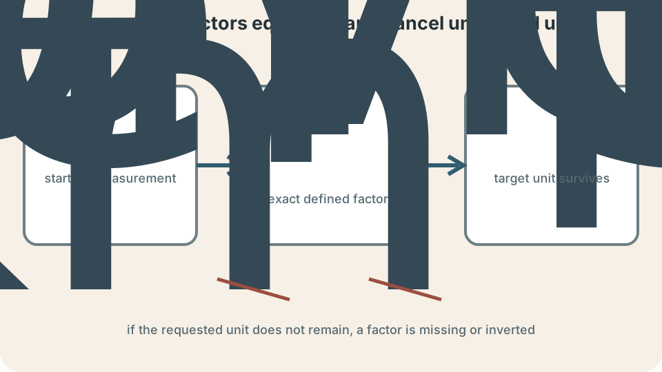
A conversion factor is a ratio of equivalent quantities and therefore equals one. Because $100\,\mathrm{cm}=1\,\mathrm m$, both $\frac{100\,\mathrm{cm}}{1\,\mathrm m}$ and its reciprocal equal one. Choose the orientation that cancels the starting unit. Units crossed out algebraically show the conversion path. The surviving unit must match the target.

Convert $2.50\,\mathrm m$ to centimetres by writing $2.50\,\mathrm m\left(\frac{100\,\mathrm{cm}}{1\,\mathrm m}\right)=250\,\mathrm{cm}$. Metres cancel between numerator and denominator. The defined factor contributes no measurement uncertainty. The starting value has three significant figures. Scientific notation can make the retained precision clearer as $2.50\times10^2\,\mathrm{cm}$.

Multi-step conversions form a chain. To convert $72.0\,\mathrm{\frac{km}{h}}$ to metres per second, multiply by $\frac{10^3\,\mathrm m}{1\,\mathrm{km}}$ and $\frac{1\,\mathrm h}{3600\,\mathrm s}$. Kilometres and hours cancel, leaving $\mathrm{\frac{m}{s}}$. The result is $20.0\,\mathrm{\frac{m}{s}}$. Writing units at every step makes an inverted factor visible.

Measurement includes uncertainty

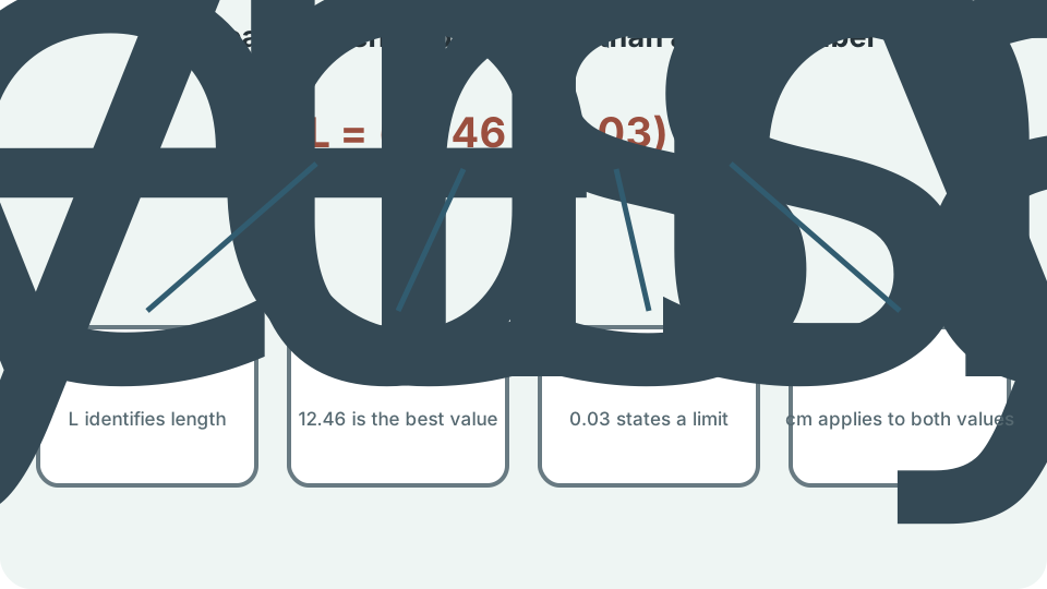
No ordinary measurement determines an exact continuous value. Instrument resolution, calibration, environmental variation, sampling, and reading method all limit knowledge. A result may be written $x=(12.46\pm0.03)\,\mathrm{cm}$. The central value is the estimate, and $0.03\,\mathrm{cm}$ is an absolute uncertainty under the stated interpretation. The unit applies to both.

The symbol $\pm$ is read “plus or minus.” It often indicates an interval from $12.43\,\mathrm{cm}$ to $12.49\,\mathrm{cm}$ in this example, but its statistical meaning must be stated. It might represent instrument resolution, one standard deviation, a confidence interval, or another bound. Different meanings are not interchangeable. The same numerical width can therefore support different probability interpretations. Good reporting names the convention.

Uncertainty is not an admission of careless work. It quantifies the limits of available information. Smaller uncertainty can support finer distinctions, but zero uncertainty is generally inappropriate for a measured continuous quantity. Exact counts and definitions are special cases. Scientific trust improves when limitations are visible.

Accuracy, precision, resolution, and error differ

Accuracy describes closeness to a reference or accepted value. Precision describes the spread or repeatability of results. A set of measurements can be tightly clustered yet displaced from the reference. That pattern is precise but inaccurate. Another set can average near the reference while individual values scatter widely.

Resolution is the smallest displayed or discernible increment of an instrument. A digital balance reading to $0.001\,\mathrm g$ has finer display resolution than one reading to $0.1\,\mathrm g$. Resolution does not guarantee accuracy at that level. Calibration bias, drift, and sample handling may dominate. Display digits are not automatic evidence of truth.

Measurement error is the difference between a measured value and an appropriate reference value. Random error changes unpredictably across repeated measurements and contributes to spread. Systematic error shifts results consistently through calibration or method bias. Repetition can reduce uncertainty in a mean affected by random variation. Repetition alone does not remove systematic bias.

Significant figures encode reported resolution

Significant figures include all certain digits reported from a measurement plus one estimated digit under a traditional analog-reading convention. In $12.40\,\mathrm g$, the trailing zero communicates precision to the hundredths place. Writing $12.4\,\mathrm g$ communicates only tenths. The two numbers have the same approximate magnitude but different reported resolution. Zeros can therefore carry information.

All nonzero digits are significant. Zeros between nonzero digits are significant, so $1002$ has four significant figures. Leading zeros only locate the decimal point, so $0.00450$ has three significant figures. Trailing zeros to the right of a decimal point are significant. Trailing zeros in a whole number without notation can be ambiguous.

Scientific notation removes that ambiguity. Writing $1.20\times10^3$ clearly gives three significant figures. Writing $1.2\times10^3$ gives two, and $1.200\times10^3$ gives four. The exponent changes scale but does not count as a significant digit. Coefficient digits communicate the reported precision.

Exact quantities do not limit precision

Counted quantities are exact when every item is known. Twelve eggs in a carton is exactly twelve under the stated count. There is no rounding uncertainty from the integer count itself. A defined conversion such as $1\,\mathrm{min}=60\,\mathrm s$ is also exact. Exact numbers have effectively unlimited significant figures in calculations.

Measured conversion factors are not exact merely because they appear in a table. A material density obtained experimentally carries uncertainty. A calibration coefficient may also be measured. The source and definition determine exactness. Never classify a number as exact solely because it lacks an uncertainty label.

Constants in defined SI relationships can be exact, while empirical constants are uncertain. The speed of light in vacuum has an exact defined SI value. A locally measured gravitational acceleration is not exact and varies with location. Context controls treatment. Documentation should distinguish definitions from observations.

Multiplication and division use relative precision

The traditional significant-figure rule for multiplication and division limits the result to the smallest number of significant figures among measured inputs. For $\rho=\frac{19.35\,\mathrm g}{2.50\,\mathrm{mL}}$, the mass has four significant figures and volume has three. The calculator gives $7.74\,\mathrm{\frac{g}{mL}}$ after appropriate rounding. The result therefore has three significant figures. Units remain in fractional form.

The deeper reason involves relative uncertainty. In a product or quotient, fractional uncertainties combine rather than absolute decimal places. A value known to about one part in one hundred should not create a product known to one part in one million. Significant-figure counting approximates this idea. Explicit uncertainty propagation is more informative when uncertainties are known.

Do not round every intermediate result. Keep guard digits through the calculation and round once at the end. Repeated rounding can shift the final value. Store full calculator precision or at least several extra digits. Present only the justified final digits.

Addition and subtraction use decimal place

For addition and subtraction, the limiting factor is the least precise decimal place, not the fewest significant figures. Consider $12.11\,\mathrm g+0.3\,\mathrm g=12.41\,\mathrm g$ before rounding. The second measurement is known only to tenths. The reported sum is therefore $12.4\,\mathrm g$. Hundredths are unsupported by that input.

This rule reflects absolute uncertainty. Adding a quantity uncertain by roughly $0.1\,\mathrm g$ to one uncertain by roughly $0.01\,\mathrm g$ leaves the sum limited mainly by tenths. Significant-figure counts alone would miss the relevant place value. Align decimal points before deciding. Then round only the result.

Mixed calculations require attention to operation order. Mark the limiting decimal place for addition or subtraction without prematurely rounding. Carry guard digits into later multiplication or division. Apply the final reporting rule after the complete calculation. A written uncertainty analysis is preferable for high-stakes work.

Rounding requires a declared convention

Standard classroom rounding examines the first discarded digit. If it is greater than five, increase the last retained digit. If it is less than five, leave the retained digit unchanged. If it is exactly five followed by nonzero digits, round upward because the discarded part exceeds half. An exact tie requires a stated tie-breaking convention.

Round-half-to-even makes the last retained digit even in an exact tie. This reduces directional bias across many repeated rounded values. Round-half-up is another common classroom convention. Software and instruments may implement different rules. Reproducible work names the convention when ties can matter.

Rounding changes a representation, not the underlying measured object. Writing more zeros after a calculation cannot create information. Writing too few digits can discard useful information. The reported precision should match uncertainty and purpose. Archive raw data at higher resolution when possible.

Absolute and relative uncertainty answer different questions

Absolute uncertainty uses the same unit as the measured quantity. If $L=(25.0\pm0.2)\,\mathrm{cm}$, the absolute uncertainty is $0.2\,\mathrm{cm}$. Relative uncertainty is the ratio $\frac{u_L}{L}$. Here it is $\frac{0.2\,\mathrm{cm}}{25.0\,\mathrm{cm}}=0.008$. Units cancel, so relative uncertainty is dimensionless.

Percentage uncertainty multiplies the relative uncertainty by $100\%$. The example gives $0.8\%$. Relative measures allow fair comparison across different scales. An absolute uncertainty of $0.2\,\mathrm{cm}$ is minor for a long object but enormous for a submillimetre feature. Context determines adequacy.

Uncertainty is commonly reported with one or two significant figures. The measured value is then rounded to the same decimal place as its absolute uncertainty. Thus $(12.4637\pm0.0321)\,\mathrm{cm}$ might become $(12.464\pm0.032)\,\mathrm{cm}$ under a stated convention. Different fields use different reporting standards. Consistency matters more than an unsupported universal rule.

Propagation estimates output uncertainty

For a sum or difference $z=x\pm y$ with independent uncertainties, a common standard-uncertainty rule is $u_z=\sqrt{u_x^2+u_y^2}$. The symbols $u_x$, $u_y$, and $u_z$ are uncertainties in the respective quantities. Squaring prevents positive and negative deviations from canceling. The square root returns the original unit. Independence is an assumption.

For a product $z=xy$ with independent small uncertainties, relative uncertainty is approximated by $\left(\frac{u_z}{z}\right)^2=\left(\frac{u_x}{x}\right)^2+\left(\frac{u_y}{y}\right)^2$. Each fraction is dimensionless. The rule extends to quotients with the same squared relative terms. Correlated inputs require covariance terms. Blindly applying the independent rule can misstate uncertainty.

For a general function $z=f(x)$, a first-order estimate is $u_z\approx\left|\frac{df}{dx}\right|u_x$. The derivative measures sensitivity of output to input. Its unit converts input uncertainty into output uncertainty. This local linear approximation works best when uncertainty is small and the function is smooth. Monte Carlo or nonlinear methods may be needed otherwise.

Worked measurement example

Suppose a rectangular sample has length $L=(5.20\pm0.02)\,\mathrm{cm}$, width $W=(2.10\pm0.01)\,\mathrm{cm}$, and thickness $T=(0.500\pm0.005)\,\mathrm{cm}$. Its volume is $V=LWT$. The central value is $(5.20)(2.10)(0.500)=5.46\,\mathrm{cm^3}$. Every input and the output retain units. The calculation assumes the sample is adequately modeled as a rectangular prism.

Assuming independent uncertainties, calculate the squared relative terms. They are $\left(\frac{0.02}{5.20}\right)^2$, $\left(\frac{0.01}{2.10}\right)^2$, and $\left(\frac{0.005}{0.500}\right)^2$. Their square root gives relative uncertainty approximately $0.0117$. Multiplying by $5.46\,\mathrm{cm^3}$ gives absolute uncertainty about $0.064\,\mathrm{cm^3}$. A reasonable report is $V=(5.46\pm0.06)\,\mathrm{cm^3}$.

The simple significant-figure rule would also report about three significant figures. The explicit propagation adds more information by showing which measurement dominates. Thickness has the largest relative uncertainty at $1.0\%$. Improving thickness measurement would therefore reduce volume uncertainty most efficiently. Measurement design follows from the uncertainty budget.

Common mistakes and repairs

One mistake is omitting units during substitution and adding them only at the end. This hides inverted conversions and dimensionally impossible operations. Carry units with every numerical value. Cancel them explicitly. Reject any result whose dimension disagrees with the requested quantity.

Another mistake is treating significant figures as a mechanical digit game. A calculator display is not a measurement. Exact counts do not constrain digits, and measured constants can. Connect every rounding choice to the least precise input or to propagated uncertainty. Preserve guard digits until the final report.

A third mistake is using “human error” as an uncertainty category. Mistakes such as recording the wrong sample should be corrected, not incorporated as random uncertainty. Identify specific sources such as calibration bias, reading resolution, temperature variation, sampling, or repeatability. Estimate their effects transparently. A useful uncertainty statement points toward improved measurement.

A reliable reporting workflow

First define the measurand, which is the quantity intended to be measured. Record the instrument, unit, resolution, calibration status, conditions, and repeated observations. Preserve raw values before rounding. Identify exact constants separately. This establishes traceability.

Second calculate with units and guard digits. Use dimensional analysis for conversions. Apply a justified uncertainty model and state assumptions such as independence. Check scale, sign, and physical plausibility. Compare alternative methods when practical.

Third report the estimate and uncertainty together. Round them consistently and state the uncertainty meaning. Include units in fractional or powered form as appropriate. Distinguish precision from accuracy and disclose important systematic limitations. A reader should be able to reconstruct what the digits claim.

Retrieval practice and synthesis

Convert $3.60\,\mathrm{\frac{g}{cm^3}}$ to $\mathrm{\frac{kg}{m^3}}$ using explicit conversion factors. Cube the length conversion because volume is cubed. Show unit cancellation before multiplying numbers. Preserve three significant figures from the measured starting density. The result is $3.60\times10^3\,\mathrm{\frac{kg}{m^3}}$.

Explain why $12.0\,\mathrm{mL}$ and $12\,\mathrm{mL}$ do not communicate identical precision. Identify the decimal place implied by each notation. Then state why neither notation alone supplies a complete statistical uncertainty. Give a possible uncertainty statement for an instrument reading. Connect the final digit to measurement resolution.

Design an uncertainty improvement for the rectangular-volume example. Compare the relative uncertainties of length, width, and thickness. Identify the dominant contribution. Propose an instrument or method that reduces it. Predict how the propagated result changes without pretending all other limitations disappear.