Buffers and Titrations

Many chemical systems must tolerate small acid or base inputs without undergoing a large pH change. Blood, cells, natural waters, foods, and laboratory solutions use conjugate acid–base chemistry to moderate those changes. A buffer accomplishes this moderation by containing substantial amounts of a weak acid and its conjugate base, or a weak base and its conjugate acid. A titration deliberately adds a measured reagent and moves the composition through several chemically distinct regions. Understanding both topics requires deciding when stoichiometric reaction occurs and when equilibrium determines the remaining composition.

You will explain buffer action at particle level, derive and use the Henderson–Hasselbalch relation, distinguish buffer range from capacity, and analyze strong-acid/strong-base and weak-acid/strong-base titrations. You will identify initial, buffer, half-equivalence, equivalence, and post-equivalence regions. You will also distinguish equivalence point from indicator endpoint and select an indicator rationally. Every logarithm, ratio, concentration, and volume will be interpreted with units. The central habit is to complete any essentially quantitative neutralization before solving the equilibrium that follows.

Begin each problem by listing actual species and moles after mixing. Determine whether an added strong acid or base reacts stoichiometrically with a buffer component or analyte. Use a mole ledger to find what remains and what forms, then divide by total volume only when concentration is needed. Identify the controlling equilibrium for that region and test whether an approximation applies. Finally, check that the predicted pH direction and magnitude fit the composition.

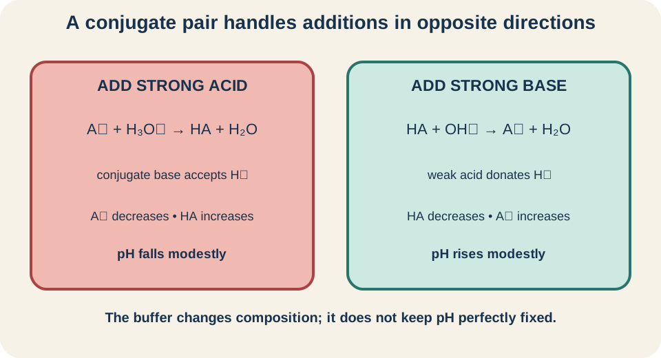
A buffer contains complementary proton-handling species

For a weak acid buffer, the pair is a weak acid $\mathrm{HA}$ and its conjugate base $\mathrm{A^-}$. The acid can donate a proton when base is added, while the conjugate base can accept a proton when acid is added. The two species differ by exactly one $\mathrm{H^+}$. Both must be present in substantial amount. A lone weak acid solution has some buffering behavior near its equilibrium composition but is not the robust mixed pair usually intended by the term buffer.

When strong acid is added, the important reaction is $\mathrm{A^-+H_3O^+\longrightarrow HA+H_2O}$. Conjugate base consumes much of the added hydronium and becomes weak acid. When strong base is added, the important reaction is $\mathrm{HA+OH^-\longrightarrow A^-+H_2O}$. Weak acid consumes much of the hydroxide and becomes conjugate base. The additions change the pair ratio rather than allowing the full strong reagent concentration to remain.

A weak base buffer works analogously with $\mathrm B$ and $\mathrm{HB^+}$. Added acid reacts with B to form $\mathrm{HB^+}$, while added base reacts with $\mathrm{HB^+}$ to form B. The names “acidic buffer” and “basic buffer” often refer to operating pH rather than to whether the pair can handle both directions. Every buffer contains an acid member and a base member. Its chosen conjugate pair sets the useful pH region.

Buffering means resistance, not constant pH

A buffer reduces the pH change caused by a given small addition compared with unbuffered water of similar volume. It does not hold pH exactly constant. Added acid converts some conjugate base into weak acid, changing their ratio. Added base converts some weak acid into conjugate base. Because pH depends logarithmically on that ratio, modest ratio changes often produce modest pH changes.

Buffer action has finite capacity. If enough strong acid is added to consume nearly all $\mathrm{A^-}$, the buffer can no longer remove additional acid effectively. If enough strong base consumes nearly all HA, base buffering is lost. Larger total amounts of both components provide greater capacity at the same ratio. A tiny-volume dilute buffer and a large-volume concentrated buffer can share pH but not capacity.

Dilution illustrates the difference. Diluting both HA and $\mathrm{A^-}$ by the same factor leaves their concentration ratio approximately unchanged, so ideal Henderson–Hasselbalch pH changes little. Yet the diluted solution contains fewer buffer moles per unit volume and has lower capacity against a fixed added amount. Activity coefficients and water autoionization can also matter at extreme dilution. Constant ratio does not imply unchanged resistance under every condition.

Derive Henderson–Hasselbalch from acid equilibrium

For $\mathrm{HA+H_2O\rightleftharpoons H_3O^++A^-}$, the idealized acid expression is $K_a=\frac{[\mathrm{H_3O^+}][\mathrm{A^-}]}{[\mathrm{HA}]}$. Rearranging gives $[\mathrm{H_3O^+}]=K_a\frac{[\mathrm{HA}]}{[\mathrm{A^-}]}$. Taking negative base-ten logarithms converts multiplicative relationships into additive ones. By definition, $\mathrm{pH}=-\log_{10}[\mathrm{H_3O^+}]$ in the common concentration shorthand and $\mathrm{p}K_a=-\log_{10}K_a$. The rigorous thermodynamic definitions use dimensionless activities.

Applying logarithm rules gives $\mathrm{pH}=\mathrm{p}K_a+\log_{10}\left(\frac{[\mathrm{A^-}]}{[\mathrm{HA}]}\right)$. The horizontal fraction bar places conjugate-base concentration over weak-acid concentration. Because numerator and denominator have the same unit $\frac{\mathrm{mol}}{\mathrm L}$, their ratio is dimensionless. The logarithm must act on a dimensionless quantity. The equation is a rearranged equilibrium relation rather than a separate law.

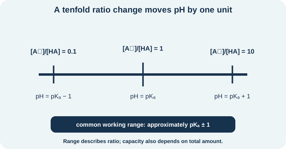
If $[\mathrm{A^-}]=[\mathrm{HA}]$, their ratio is one and $\log_{10}(1)=0$. Therefore $\mathrm{pH}=\mathrm{p}K_a$. If base is ten times acid, the logarithm is one and pH is one unit above $\mathrm{p}K_a$. If base is one-tenth acid, the logarithm is negative one and pH is one unit below $\mathrm{p}K_a$. These landmarks make ratio effects intuitive.

Know the assumptions behind the buffer equation

The Henderson–Hasselbalch form assumes that activities can be represented adequately by concentration ratios or that activity effects cancel sufficiently for the task. It also presumes both conjugate components are present and that their equilibrium changes are small relative to their prepared amounts. At high ionic strength, activity coefficients can shift the relationship. At extreme dilution, water autoionization can become important. The compact equation is a model with a domain.

The relation should not be applied before stoichiometric neutralization with an added strong acid or base. Strong reagent first consumes the appropriate buffer component essentially quantitatively. Only the remaining conjugate pair enters the ratio. Using initial amounts would ignore the chemical reaction caused by the addition. A mole ledger must precede equilibrium evaluation.

Concentration ratios can often be replaced by mole ratios after mixing because both species occupy the same total solution volume. Specifically, $\frac{[\mathrm{A^-}]}{[\mathrm{HA}]}=\frac{n_{\mathrm{A^-}}/V}{n_{\mathrm{HA}}/V}=\frac{n_{\mathrm{A^-}}}{n_{\mathrm{HA}}}$. The common volume $V$ cancels. This simplification is valid only when both concentrations refer to that same final volume. Keeping the derivation visible prevents cancellation across unlike solutions before mixing.

Buffer range and buffer capacity are different

A common practical buffer range is approximately $\mathrm{p}K_a\pm1$. Within this interval, the conjugate-base-to-acid ratio lies between about $0.1$ and $10$. Both components remain appreciable enough to respond in their respective directions. This guideline follows directly from the logarithmic relation. It is not a sharp boundary where buffering suddenly switches off.

Buffer capacity measures how much strong acid or base can be added before pH changes substantially. It increases with total concentration of the conjugate pair and is greatest near comparable component amounts for balanced two-direction resistance. Two buffers can have identical pH and ratio but different total concentrations. The more concentrated buffer has greater capacity. Volume also affects total moles available to neutralize an addition.

Choosing a buffer therefore requires both a suitable $\mathrm{p}K_a$ and enough material. Select a conjugate pair whose $\mathrm{p}K_a$ is near the target pH, then choose component ratio using Henderson–Hasselbalch. Determine total concentration and volume from expected acid or base load and acceptable pH change. Consider compatibility, toxicity, temperature, and ionic strength in real applications. A ratio calculation alone is not a complete design.

A buffer calculation begins with a mole ledger

Suppose $1.00\,\mathrm L$ contains $0.200\,\mathrm{mol}$ HA and $0.200\,\mathrm{mol}$ $\mathrm{A^-}$, with $\mathrm{p}K_a=4.76$. Initially the ratio is one, so pH is $4.76$ in the ideal model. Add $0.0100\,\mathrm{mol}$ strong acid while treating volume change as negligible. Hydronium consumes $0.0100\,\mathrm{mol}$ $\mathrm{A^-}$ and creates the same amount HA. The new amounts are $0.190\,\mathrm{mol}$ base and $0.210\,\mathrm{mol}$ acid.

Use the post-reaction ratio: $\mathrm{pH}=4.76+\log_{10}\left(\frac{0.190}{0.210}\right)$. The ratio is approximately $0.905$, whose base-ten logarithm is about $-0.043$. The new pH is approximately $4.72$. The strong acid addition lowered pH, but the change is modest because the buffer converted acid input into weak acid. The sign and scale both fit the particle model.

If the same acid amount were added to unbuffered pure water, a simple strong-acid model in roughly one liter would give hydronium near $0.0100\,\frac{\mathrm{mol}}{\mathrm L}$ and pH near $2.00$. That comparison illustrates resistance rather than perfect constancy. Exact results would account for final volume and activities. The buffer’s success depends on its much larger available conjugate-base amount. Capacity would eventually fail if additions approached that amount.

Titration measures composition through controlled addition

A titration adds a solution of known concentration, called the titrant, to an analyte solution. The delivered titrant volume is measured, and the reaction stoichiometry relates titrant moles to analyte moles. Acid–base titrations often monitor pH as volume is added. The resulting titration curve reveals chemically distinct regions. No single pH formula applies across the entire curve.

Moles of a dissolved titrant are calculated as $n=CV$, where $C$ is molar concentration and $V$ is volume in liters. A concentration of $0.100\,\frac{\mathrm{mol}}{\mathrm L}$ delivered in $0.0250\,\mathrm L$ provides $0.00250\,\mathrm{mol}$. Liters cancel through the product. Milliliters must be converted to liters before using these units. The balanced neutralization equation determines the mole ratio to analyte.

The equivalence point occurs when stoichiometrically equivalent amounts have reacted according to the balanced equation. It does not universally mean pH seven. Strong-acid/strong-base equivalence is near neutral at ordinary temperature under ideal assumptions, but weak-acid/strong-base equivalence is basic because the conjugate base hydrolyzes. Weak-base/strong-acid equivalence is acidic for the analogous reason. Chemistry of the equivalence mixture controls pH.

Strong-acid/strong-base titration is controlled by excess reagent

For monoprotic strong acid titrated with strong base, the net ionic reaction is $\mathrm{H_3O^++OH^-\longrightarrow2H_2O}$. Before equivalence, hydronium is in excess and determines pH after dilution. Calculate initial hydronium moles, subtract added hydroxide moles, and divide remaining hydronium by total volume. Then compute pH from the resulting concentration. Stoichiometry comes before logarithms.

At equivalence, neither strong reagent remains in stoichiometric excess. The solution contains water and spectator ions from the acid and base. Under a simple $25\,\mathrm{^{\circ}C}$ ideal model with neutral spectators, water autoionization gives pH near $7.00$. Temperature matters because $K_w$ changes. Spectator-ion chemistry can also invalidate the simplest neutral assumption.

After equivalence, hydroxide is in excess. Subtract consumed hydroxide from delivered hydroxide, divide the excess by total volume, and calculate pOH. At $25\,\mathrm{^{\circ}C}$ under the familiar ideal model, $\mathrm{pH}+\mathrm{pOH}=14.00$. The number fourteen is temperature-dependent through $\mathrm{p}K_w$. Excess strong titrant dominates far enough beyond equivalence.

Weak-acid/strong-base titration changes controlling models

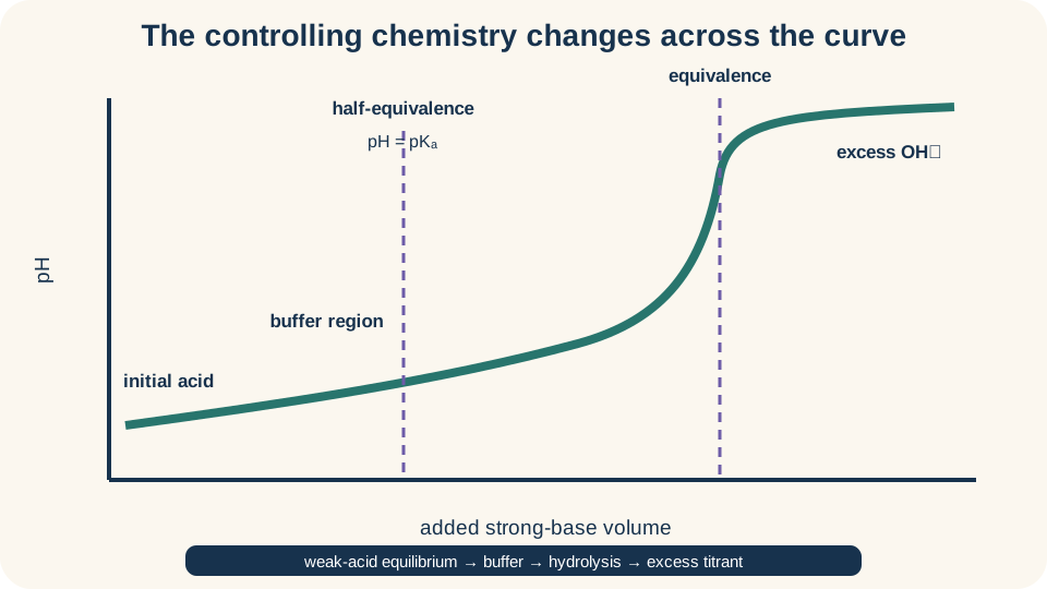
At the initial point, only weak acid and its acid-ionization equilibrium determine pH. A $K_a$ calculation, often using an ICE table, is appropriate. After some strong base is added but before equivalence, stoichiometric neutralization creates conjugate base while leaving weak acid. The mixture is then a buffer. Henderson–Hasselbalch can apply after the mole ledger is updated.

At half-equivalence, added base has converted exactly half the initial acid into conjugate base. Remaining HA moles equal formed $\mathrm{A^-}$ moles, so their ratio is one. Therefore $\mathrm{pH}=\mathrm{p}K_a$. This point provides an experimental route to estimate $\mathrm{p}K_a$ from a titration curve. Half-equivalence refers to half the equivalence volume for fixed titrant concentration and one-to-one stoichiometry.

At equivalence, the original weak acid has been converted into conjugate base. Henderson–Hasselbalch cannot be used with zero remaining HA in its ratio. Instead, conjugate-base hydrolysis $\mathrm{A^-+H_2O\rightleftharpoons HA+OH^-}$ controls pH. Use $K_b=\frac{K_w}{K_a}$ for the conjugate pair and the formal conjugate-base concentration after dilution. Beyond equivalence, excess strong hydroxide becomes the primary pH controller.

Work a weak-acid titration by regions

Suppose $25.00\,\mathrm{mL}$ of $0.1000\,\frac{\mathrm{mol}}{\mathrm L}$ monoprotic weak acid is titrated with $0.1000\,\frac{\mathrm{mol}}{\mathrm L}$ strong base. Initial acid amount is $0.1000\,\frac{\mathrm{mol}}{\mathrm L}\times0.02500\,\mathrm L=0.002500\,\mathrm{mol}$. One-to-one stoichiometry requires the same hydroxide amount at equivalence. The equivalence volume is therefore $0.02500\,\mathrm L$ or $25.00\,\mathrm{mL}$. This result follows from stoichiometry, not from a pH measurement.

At $12.50\,\mathrm{mL}$ added base, hydroxide moles are $0.001250\,\mathrm{mol}$, exactly half the initial acid amount. Neutralization leaves $0.001250\,\mathrm{mol}$ HA and creates $0.001250\,\mathrm{mol}$ $\mathrm{A^-}$. The ratio is one, so pH equals $\mathrm{p}K_a$. Total volume cancels from the ratio because both components share it. This is the half-equivalence landmark.

At equivalence, calculate the concentration of $\mathrm{A^-}$ using total volume $50.00\,\mathrm{mL}=0.05000\,\mathrm L$. The formal concentration is $\frac{0.002500\,\mathrm{mol}}{0.05000\,\mathrm L}=0.05000\,\frac{\mathrm{mol}}{\mathrm L}$. This value becomes the initial conjugate-base concentration for a hydrolysis equilibrium. The pH is above seven for an ordinary weak-acid/strong-base pair at $25\,\mathrm{^{\circ}C}$. A numerical value requires the original acid’s $K_a$.

Equivalence point and endpoint are not identical concepts

The equivalence point is a stoichiometric condition defined by reacting amounts. The endpoint is an observed experimental signal used to estimate that condition. An indicator endpoint may be a persistent color change, while an instrumental endpoint may be inferred from a pH-curve feature. The two should be close for a well-designed titration. They are not definitionally the same point.

An acid–base indicator is itself a weak acid–base system whose forms have different colors. Its transition occurs over a pH interval related to its own $\mathrm{p}K_a$. Choose an indicator whose transition range lies within the steep pH change near the titration’s equivalence point. Phenolphthalein may suit some weak-acid/strong-base titrations because their equivalence region is basic. A low-pH indicator could signal too early.

Indicator error is the titrant-volume difference between the observed endpoint and true equivalence under the method. Adding too much titrant after a persistent endpoint overshoots. Using excessive indicator can also perturb a small or weakly buffered sample because indicator is chemically active. Instrumental curves reduce reliance on visual color judgment but still require calibration and interpretation. Experimental design connects chemical theory to measurement quality.

Titration curves encode capacity and composition

The slope of a titration curve indicates how strongly pH responds to added volume. Buffer regions are relatively shallow because conjugate components absorb additions through conversion. Near equivalence, one buffer component becomes depleted and pH can change steeply with small titrant additions. Beyond equivalence, the curve reflects dilution and excess strong titrant. Shape therefore records changing chemical control.

The equivalence volume reveals analyte amount through stoichiometry. The half-equivalence pH reveals $\mathrm{p}K_a$ for a monoprotic weak acid under appropriate assumptions. The initial pH constrains acid strength and concentration. Multiple equivalence regions can suggest polyprotic behavior when successive proton transfers are sufficiently separated. A curve is a dataset, not merely a picture of “going upward.” Each extracted feature should be tied to a chemical region and measurement uncertainty.

Derivative methods can locate inflection features in instrumental data, but noise and sampling density affect them. The first derivative approximates slope change per volume, while the second derivative can identify curvature changes. These numerical tools do not replace chemical validation of reaction stoichiometry. Temperature, ionic strength, electrode response, and mixing all affect the measured curve. Interpretation should join computation with experimental context.

Common errors and corrective habits

The most common calculation error is applying an equilibrium formula before completing strong neutralization. Build an initial–reaction–remaining mole ledger first. Another error is using initial solution volume instead of total mixed volume for post-addition concentrations. Add analyte and titrant volumes unless a justified approximation says otherwise. Keep milliliters and liters consistent.

A second error is using Henderson–Hasselbalch at equivalence when one buffer component has been consumed. Switch to conjugate-species hydrolysis. A third error is assuming equivalence pH is always seven. Identify the salt ions and test their acid–base behavior. The reaction partners determine equivalence chemistry.

A conceptual error treats buffer pH and capacity as the same property. Ratio largely controls ideal pH, while total component amounts control capacity. Another treats endpoint and equivalence as synonyms. State which is theoretical and which is observed. A final check should name the controlling species and equation in the region being calculated.

Guided practice and retrieval

A buffer contains $0.300\,\mathrm{mol}$ HA and $0.150\,\mathrm{mol}$ $\mathrm{A^-}$ with $\mathrm{p}K_a=5.00$. The ratio is $\frac{0.150}{0.300}=0.500$. Therefore pH is $5.00+\log_{10}(0.500)\approx4.70$. The pH lies below $\mathrm{p}K_a$ because proton-donating HA exceeds proton-accepting $\mathrm{A^-}$. State why the common solution volume cancels.

If $0.050\,\mathrm{mol}$ hydroxide is added, it consumes HA and produces $\mathrm{A^-}$. New amounts are $0.250\,\mathrm{mol}$ HA and $0.200\,\mathrm{mol}$ $\mathrm{A^-}$. The new ratio is $0.800$, producing pH approximately $4.90$ under the model. The pH rises, as expected when base is added. Using the original ratio would miss the neutralization.

For a weak-acid/strong-base titration, list the controlling method in order. Initial solution uses weak-acid equilibrium, the pre-equivalence mixture uses stoichiometry followed by buffer equilibrium, half-equivalence gives pH equal to $\mathrm{p}K_a$, equivalence uses conjugate-base hydrolysis, and post-equivalence uses excess hydroxide. Each region requires a different inventory. Memorizing one equation for the whole curve cannot work. Naming the surviving species is the fastest way to select the correct model.

Connection forward

Reconstruct buffer action at particle level. Explain how each conjugate component responds to added strong acid or base, derive Henderson–Hasselbalch from $K_a$, and distinguish pH range from capacity. Then walk through every titration region and state which calculation comes first. Define equivalence and endpoint separately. If a numerical method is named without a controlling species, revisit the composition ledger.

Reaction quotients and Le Châtelier reasoning will explain the direction of buffer equilibrium adjustments after disturbance. Solubility and complex-ion titrations reuse the sequence of stoichiometry followed by equilibrium. Analytical chemistry extends endpoint detection, uncertainty, calibration, and curve fitting. Biological systems add multiple coupled buffers and open-system gas exchange. The foundational conjugate-pair ledger remains useful in all of them.

The enduring framework is staged reasoning. Strong neutralization changes amounts first, equilibrium distributes the remaining weak species second, and a logarithm reports hydronium activity last. Buffers resist rather than forbid pH change, and their capacity depends on material amount. Titration regions change because the surviving species change. Once the inventory is made explicit, formula choice follows from chemistry instead of guesswork.