Numerical Integration and Error

Overview

Central question: What can we know when an elementary antiderivative is unavailable? You will build an integral estimate from sampled data, select a numerical model that matches the available information, and state what kind of error remains. The important distinction is between an exact accumulated quantity and an approximation whose assumptions are visible.

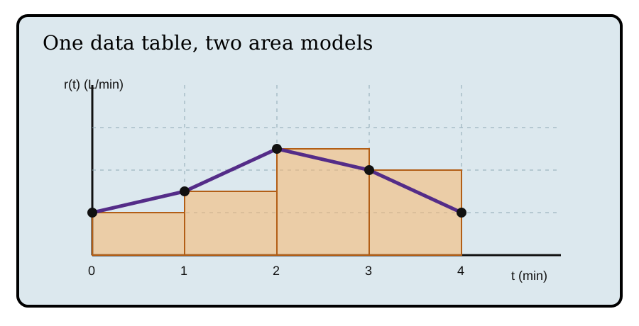
Imagine a flow meter reporting values once each minute. It does not reveal the entire curve between readings, but the water still moves continuously. Before using a formula, decide what a rectangle drawn from one reading is claiming about the unobserved part of the graph. Does its height describe the beginning, end, or a representative point of the interval? That decision determines the estimate.

From samples to accumulated change

Suppose a rate $r(t)$ , measured in $\frac{\mathrm L}{\mathrm{min}}$ , is recorded at one-minute intervals:

$t$ (min)	0	1	2	3	4
$r(t)$ (L/min)	2	3	5	4	2

The target $\int_0^{4\,\mathrm{min}}r(t)\,dt$ has units of liters because each small product $r(t)\,dt$ combines rate with time. A left sum uses the values at $t=0,1,2,3$ as rectangle heights. Its estimate is

L_4=(2+3+5+4)\,\frac{\mathrm L}{\mathrm{min}} \left(1\,\mathrm{min}\right)=14\,\mathrm L.

L5-V01 - Rectangle and trapezoid comparison. Place this beside the first calculation. It is a static graph with time in minutes on the horizontal axis and rate in Lmin\frac{\mathrm L}{\mathrm{min}}minL on the vertical axis; it uses the five tabulated points, four left rectangles, and four connecting trapezoids on the same scale. Its purpose is to show that every numerical method adds model areas, not raw data values

Four measured rate points support both left rectangles and connecting trapezoids; each shape estimates accumulated liters over a one-minute interval.

A different geometric promise

The trapezoidal rule replaces the unknown curve between two readings by the straight segment joining them. With equally spaced readings, its estimate is

T_4=\frac{1\,\mathrm{min}}{2} \left[2+2(3)+2(5)+2(4)+2\right] \frac{\mathrm L}{\mathrm{min}} =14\,\mathrm L.

The numerical coincidence $L_4=T_4$ does not prove that the true accumulated volume is exactly $14\,\mathrm L$ . It says only that these two different approximations agree for this data. If the true curve bows above or below a trapezoid between readings, the trapezoid has error; the sign of that error depends on concavity.

There is also a modeling decision hidden in the word “data.” A table may contain measurement error, rounded values, or values averaged over a short interval rather than instantaneous rates. Numerical integration cannot undo those limitations. It answers a narrower, honest question: given these values and this interpolation model, what accumulated value does the model predict? This is why a final report should identify the method and give a precision that matches the measurements, rather than presenting every calculator digit as physical knowledge.

L5-V02 - Curvature and trapezoid error. Place this directly after the preceding paragraph. It is a two-panel static graph with the same labeled axes and scales: a concave-up curve with secant segments above it, and a concave-down curve with secant segments below it. Shade the error regions and label them “overestimate” and “underestimate.” Alt text: “For concave-up data trapezoids lie above the curve; for concave-down data they lie below.”

Simpson’s Rule takes a further step: over pairs of equal-width subintervals it fits a quadratic arc through three equally spaced values. It requires an even number of subintervals. For smooth functions it often improves on rectangles and trapezoids, but it is still an approximation and should not be reported with more precision than the data justify.

Test the estimate rather than worship it

Refining a partition makes the model pieces narrower. If successive estimates stabilize, that is evidence that geometric approximation error is shrinking. It is not proof that the meter is accurate, that the process is smooth, or that a sudden spike did not occur between samples. State what the data support.

For a function known to be increasing, the left and right sums provide a useful bracket: the left sum is below the true integral and the right sum is above it. For a decreasing function, the ordering reverses. This conclusion follows from the rectangle heights on each subinterval; it does not require an antiderivative. A bracket is stronger evidence than one isolated estimate because it states an interval in which the accumulated value must lie.

L5-V03 - Refinement sequence. Place this beside the refinement discussion. It is a static three-panel comparison of the same smooth rate curve with four, eight, and sixteen rectangles, all on the same axes and with the increasing number of narrow error slivers visible

Stop and check

A tempting statement is: “The trapezoidal value is exact because it used all five readings.” The misconception is treating measured points as the entire function. The correction is to name the interpolating assumption: trapezoids model straight behavior between points. The exact integral is known only if the actual function is known or if independent error bounds establish the needed precision.

Retrieval check

For an increasing rate on an interval, explain why a left sum is below the true area and a right sum is above it. Then name one fact you would need before claiming a trapezoidal estimate is an overestimate. A complete response mentions concavity, not merely whether the rate is increasing.

The next unit returns to exact symbolic work. Integration by parts begins where substitution does not: a product whose derivative structure can be traded for another, simpler integral.